torchbox.evaluation package

Submodules

torchbox.evaluation.capacity module

torchbox.evaluation.capacity.capacity(H, snr, cdim, dim=(-2, -1), keepdim=False, reduction='mean')

computes capacity of channel

MIMO-OFDM Wireless Communications with MATLAB

Parameters:

• H (Tensor) – the input channel

• snr (float) – the signal-to-noise ratio

• cdim (int or None) – If H is complex-valued, cdim is ignored. If H is real-valued and cdim is an integer then H will be treated as complex-valued, in this case, cdim specifies the complex axis.

• dim (int or None) – The dimension indexes of antenna of BS and MS. The default is (-2, -1).

• keepdim (bool) – keep dimensions? (include complex dim, defalut is False)

• reduction (str or None, optional) – The operation mode of reduction, None, 'mean' or 'sum' (the default is ‘mean’)

torchbox.evaluation.classification module

torchbox.evaluation.classification.accuracy(P, T, axis=None)

computes the accuracy

\[A = \frac{\sum(P==T)}{N} \]

where \(N\) is the number of samples.

Parameters:

• P (list or tensor) – predicted label (categorical or one-hot)

• T (list or tensor) – target label (categorical or one-hot)

• axis (int, optional) – the one-hot encoding axis, by default None, which means P and T are categorical.

Returns:

the accuracy

Return type:

float

Raises:

• ValueError – P and T should have the same shape!

• ValueError – You should specify the one-hot encoding axis when P and T are in one-hot formation!

Examples

import torchbox as tb

T = th.tensor([1, 2, 3, 4, 5, 6, 1, 2, 3, 4, 5, 6, 1, 2, 3, 4, 5, 6, 1, 5])
P = th.tensor([1, 2, 3, 4, 1, 6, 3, 2, 1, 4, 5, 6, 1, 2, 1, 4, 5, 6, 1, 5])

print(tb.accuracy(P, T))

#---output
0.8

torchbox.evaluation.classification.categorical2onehot(X, nclass=None, offset='min')

converts categorical to onehot

Parameters:

• X (list or tensor) – the categorical list or tensor

• nclass (int, optional) – the number of classes, by default None (auto detected)

• offset (int, str or None, optional) – the offset, by default 'min' (the minimum value of input)

Returns:

the one-hot matrix

Return type:

tensor

torchbox.evaluation.classification.confusion(P, T, axis=None, cmpmode='...')

computes the confusion matrix

Parameters:

• P (list or tensor) – predicted label (categorical or one-hot)

• T (list or tensor) – target label (categorical or one-hot)

• axis (int, optional) – the one-hot encoding axis, by default None, which means P and T are categorical.

• cmpmode (str, optional) – '...' for one-by one mode, '@' for multiplication mode (\(P^TT\)), by default ‘…’

Returns:

the confusion matrix

Return type:

tensor

Raises:

• ValueError – P and T should have the same shape!

• ValueError – You should specify the one-hot encoding axis when P and T are in one-hot formation!

Examples

import torchbox as tb

T = th.tensor([1, 2, 3, 4, 5, 6, 1, 2, 3, 4, 5, 6, 1, 2, 3, 4, 5, 6, 1, 5])
P = th.tensor([1, 2, 3, 4, 1, 6, 3, 2, 1, 4, 5, 6, 1, 2, 1, 4, 5, 6, 1, 5])

C = tb.confusion(P, T, cmpmode='...')
print(C)
C = tb.confusion(P, T, cmpmode='@')
print(C)

#---output
[[3. 0. 2. 0. 1. 0.]
[0. 3. 0. 0. 0. 0.]
[1. 0. 1. 0. 0. 0.]
[0. 0. 0. 3. 0. 0.]
[0. 0. 0. 0. 3. 0.]
[0. 0. 0. 0. 0. 3.]]
[[3. 0. 2. 0. 1. 0.]
[0. 3. 0. 0. 0. 0.]
[1. 0. 1. 0. 0. 0.]
[0. 0. 0. 3. 0. 0.]
[0. 0. 0. 0. 3. 0.]
[0. 0. 0. 0. 0. 3.]]

torchbox.evaluation.classification.kappa(C)

computes kappa

\[K = \frac{p_o - p_e}{1 - p_e} \]

where \(p_o\) and \(p_e\) can be obtained by

\[p_o = \frac{\sum_iC_{ii}}{\sum_i\sum_jC_{ij}} \]

\[p_e = \frac{\sum_j\left(\sum_iC_{ij}\sum_iC_{ji}\right)}{\sum_i\sum_jC_{ij}} \]

Parameters:

C (Tensor) – The confusion matrix

Returns:

The kappa value.

Return type:

float

Examples

import torchbox as tb

T = th.tensor([1, 2, 3, 4, 5, 6, 1, 2, 3, 4, 5, 6, 1, 2, 3, 4, 5, 6, 1, 5])
P = th.tensor([1, 2, 3, 4, 1, 6, 3, 2, 1, 4, 5, 6, 1, 2, 1, 4, 5, 6, 1, 5])

C = tb.confusion(P, T, cmpmode='...')
print(tb.kappa(C))
print(tb.kappa(C.T))

#---output
0.7583081570996979
0.7583081570996979

torchbox.evaluation.classification.onehot2categorical(X, axis=-1, offset=0)

converts onehot to categorical

Parameters:

• X (list or tensor) – the one-hot tensor

• axis (int, optional) – the axis for one-hot encoding, by default -1

• offset (int, optional) – category label head, by default 0

Returns:

the category label

Return type:

tensor

torchbox.evaluation.classification.plot_confusion(C, cmap=None, mode='rich', xticks='label', yticks='label', xlabel='Target', ylabel='Predicted', title='Confusion matrix', **kwargs)

plots confusion matrix.

plots confusion matrix.

Parameters:

• C (Tensor) – The confusion matrix

• cmap (None or str, optional) – The colormap, by default None, which means our default configuration (green-coral) see rgb2gray() for available colormap str.

• mode (str, optional) – 'pure', 'bare', 'simple' or 'rich'

• xticks (str, tuple or list, optional) – 'label' –> class labels, or you can specify class name list, by default 'label'

• yticks (str, tuple or list, optional) – 'label' –> class labels, or you can specify class name list, by default 'label'

• xlabel (str, optional) – The label string of axis-x, by default ‘Target’

• ylabel (str, optional) – The label string of axis-y, by default ‘Predicted’

• title (str, optional) – The title string, by default ‘Confusion matrix’

• kwargs –

  linespacingfloat

  The line spacing of text, by default 0.15

  numftddict

  The font dict of integer value, by default

  dict(fontsize=12, color='black',
       family='Times New Roman',
       weight='bold', style='normal')
  

  pctftddict

  The font dict of percent value, by default

  dict(fontsize=12, color='black',
       family='Times New Roman',
       weight='light', style='normal')
  

  restftddict

  The font dict of label, title and ticks, by default

  dict(fontsize=12, color='black',
       family='Times New Roman',
       weight='light', style='normal')
  

  pctfmtstr

  the format of percent value, such as '%.xf' means formating with two decimal places, by default '%.1f'

Returns:

pyplot handle

Return type:

pyplot

Example

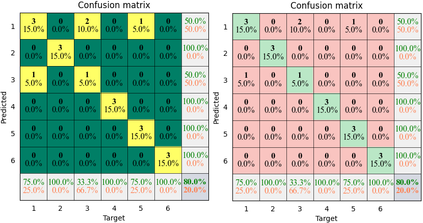
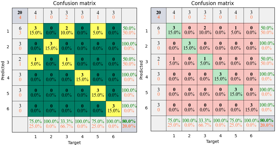
The results shown in the above figure can be obtained by the following codes.

import torchbox as tb

T = th.tensor([1, 2, 3, 4, 5, 6, 1, 2, 3, 4, 5, 6, 1, 2, 3, 4, 5, 6, 1, 5.0])
P = th.tensor([1, 2, 3, 4, 1, 6, 3, 2, 1, 4, 5, 6, 1, 2, 1, 4, 5, 6, 1, 5.0])
classnames = ['cat', 'dog', 'car', 'cup', 'desk', 'baby']

print(tb.accuracy(P, T))
print(tb.categorical2onehot(T))

C = tb.confusion(P, T, cmpmode='...')
print(C)
C = tb.confusion(P, T, cmpmode='@')
print(C)
print(tb.kappa(C))
print(tb.kappa(C.T))

plt = tb.plot_confusion(C, cmap=None, mode='pure')
plt = tb.plot_confusion(C, cmap='summer', xticks=classnames, yticks=classnames, mode='pure')
plt.show()

plt = tb.plot_confusion(C, cmap=None, mode='bare')
plt = tb.plot_confusion(C, cmap='summer', xticks=classnames, yticks=classnames, mode='bare')
plt.show()

plt = tb.plot_confusion(C, cmap=None, mode='simple')
plt = tb.plot_confusion(C, cmap='summer', xticks=classnames, yticks=classnames, mode='simple')
plt.show()

plt = tb.plot_confusion(C, cmap=None, mode='rich')
plt = tb.plot_confusion(C, cmap='summer', xticks=classnames, yticks=classnames, mode='rich')
plt.show()

torchbox.evaluation.contrast module

torchbox.evaluation.contrast.contrast(X, mode='way1', cdim=None, dim=None, keepdim=False, reduction=None)

Compute contrast of an complex image

'way1' is defined as follows, see [1]:

\[C = \frac{\sqrt{{\rm E}\left(|I|^2 - {\rm E}(|I|^2)\right)^2}}{{\rm E}(|I|^2)} \]

'way2' is defined as follows, see [2]:

\[C = \frac{{\rm E}(|I|^2)}{\left({\rm E}(|I|)\right)^2} \]

[1] Efficient Nonparametric ISAR Autofocus Algorithm Based on Contrast Maximization and Newton [2] section 13.4.1 in “Ian G. Cumming’s SAR book”

Parameters:

• X (torch tensor) – The image array.

• mode (str, optional) – 'way1' or 'way2'

• cdim (int or None) – If X is complex-valued, cdim is ignored. If X is real-valued and cdim is integer then X will be treated as complex-valued, in this case, cdim specifies the complex axis; otherwise (None), X will be treated as real-valued

• dim (tuple, None, optional) – The dimension axis for computing contrast. The default is None, which means all.

• keepdim (bool) – keep dimensions? (include complex dim, defalut is False)

• reduction (str or None, optional) – The operation mode of reduction, None, 'mean' or 'sum' (the default is None)

Returns:

C – The contrast value of input.

Return type:

scalar or tensor

Examples

th.manual_seed(2020)
X = th.randn(5, 2, 3, 4)

# real
C1 = contrast(X, cdim=None, dim=(-2, -1), mode='way1', reduction=None)
C2 = contrast(X, cdim=None, dim=(-2, -1), mode='way1', reduction='sum')
C3 = contrast(X, cdim=None, dim=(-2, -1), mode='way1', reduction='mean')
print(C1, C2, C3)

# complex in real format
C1 = contrast(X, cdim=1, dim=(-2, -1), mode='way1', reduction=None)
C2 = contrast(X, cdim=1, dim=(-2, -1), mode='way1', reduction='sum')
C3 = contrast(X, cdim=1, dim=(-2, -1), mode='way1', reduction='mean')
print(C1, C2, C3)

# complex in complex format
X = X[:, 0, ...] + 1j * X[:, 1, ...]
C1 = contrast(X, cdim=None, dim=(-2, -1), mode='way1', reduction=None)
C2 = contrast(X, cdim=None, dim=(-2, -1), mode='way1', reduction='sum')
C3 = contrast(X, cdim=None, dim=(-2, -1), mode='way1', reduction='mean')
print(C1, C2, C3)

# output
tensor([[1.2612, 1.1085],
        [1.5992, 1.2124],
        [0.8201, 0.9887],
        [1.4376, 1.0091],
        [1.1397, 1.1860]]) tensor(11.7626) tensor(1.1763)
tensor([0.6321, 1.1808, 0.5884, 1.1346, 0.6038]) tensor(4.1396) tensor(0.8279)
tensor([0.6321, 1.1808, 0.5884, 1.1346, 0.6038]) tensor(4.1396) tensor(0.8279)

torchbox.evaluation.correlation module

torchbox.evaluation.correlation.cossim(P, G, mode=None, cdim=None, dim=None, keepdim=False, reduction=None)

compute cosine similarity

\[s = \frac{<{\bf p}, {\bf g}>}{\|{\bf p}\|_2\|{\bf g}\|_2} \]

Note

For complex, the magnitude still gives the “similarity” between them, where the complex angle gives the complex phase factor required to fully reach that similarity. refers Cosine similarity between complex vectors

Parameters:

• P (Tensor) – predicted/estimated/reconstructed

• G (Tensor) – ground-truth/target

• mode (str or None) – only work when P and G are complex-valued in real format or complex format. 'abs' or 'amplitude' returns the amplitude of similarity, 'angle' or 'phase' returns the phase of similarity None returns the complex-valued similarity (default).

• cdim (int or None) – If P is complex-valued, cdim is ignored. If P is real-valued and cdim is integer then P will be treated as complex-valued, in this case, cdim specifies the complex axis; otherwise (None), P will be treated as real-valued

• dim (tuple, None, optional) – The dimension indexes for computing cosine similarity. The default is None, which means all.

• keepdim (bool) – keep dimensions? (include complex dim, defalut is False)

• reduction (str or None, optional) – The operation mode of reduction, None, 'mean' or 'sum' (the default is None)

Returns:

• S (scalar or tensor) – The cosine similarity value of inputs.

• see also peacor(), eigveccor(), CosSim, PeaCor, EigVecCor, CosSimLoss, EigVecCorLoss.

Examples

import torch as th
from torchbox import cossim

th.manual_seed(2020)
P = th.randn(5, 2, 3, 4)
G = th.randn(5, 2, 3, 4)
dim = (-2, -1)

# real
C1 = cossim(P, G, cdim=None, dim=dim, reduction=None)
C2 = cossim(P, G, cdim=None, dim=dim, reduction='sum')
C3 = cossim(P, G, cdim=None, dim=dim, reduction='mean')
print(C1, C2, C3)

# complex in real format
C1 = cossim(P, G, cdim=1, dim=dim, reduction=None)
C2 = cossim(P, G, cdim=1, dim=dim, reduction='sum')
C3 = cossim(P, G, cdim=1, dim=dim, reduction='mean')
print(C1, C2, C3)

# complex in complex format
P = P[:, 0, ...] + 1j * P[:, 1, ...]
G = G[:, 0, ...] + 1j * G[:, 1, ...]
C1 = cossim(P, G, cdim=None, dim=dim, reduction=None)
C2 = cossim(P, G, cdim=None, dim=dim, reduction='sum')
C3 = cossim(P, G, cdim=None, dim=dim, reduction='mean')
print(C1, C2, C3)

torchbox.evaluation.correlation.eigveccor(P, G, npcs=4, mode=None, cdim=None, fdim=-2, sdim=-1, keepdim=False, reduction=None)

computes cosine similarity of eigenvectors

Parameters:

• P (Tensor) – predicted/estimated/reconstructed

• G (Tensor) – ground-truth/target

• npcs (int, optional) – the number principal components for comparing, by default 4

• mode (str or None) – only work when P and G are complex-valued in real format or complex format. 'abs' or 'amplitude' returns the amplitude of similarity, 'angle' or 'phase' returns the phase of similarity None returns the complex-valued similarity (default).

• cdim (int or None) – If P and G is complex-valued, cdim is ignored. If P and G is real-valued and cdim is integer then P and G will be treated as complex-valued, in this case, cdim specifies the complex axis; otherwise (None), P and G will be treated as real-valued

• fdim (int, optional) – the dimension index of feature, by default -2

• sdim (int, optional) – the dimension index of sample, by default -1

• keepdim (bool) – keep dimensions? (include complex dim, defalut is False)

• reduction (str or None, optional) – The operation mode of reduction, None, 'mean' or 'sum' (the default is None)

Returns:

• S (scalar or tensor) – The eigenvector correlation value of inputs.

• see also cossim(), peacor(), CosSim, PeaCor, EigVecCor, CosSimLoss, EigVecCorLoss.

Examples

import torch as th
from torchbox import eigveccor

print('---compare eigen vector correlation (complex in real)')
G = th.randn(2, 3, 2, 64, 4)
P = th.randn(2, 3, 2, 64, 4)
print(eigveccor(G, G, npcs=4, cdim=2, sdim=-1, fdim=-2, keepdim=False, reduction='mean'))
print(eigveccor(G, G, npcs=4, cdim=2, sdim=-1, fdim=-2, keepdim=False, reduction=None).shape)

print('---compare eigen vector correlation (complex in complex)')
G = th.randn(2, 3, 64, 4) + 1j*th.randn(2, 3, 64, 4)
P = th.randn(2, 3, 64, 4) + 1j*th.randn(2, 3, 64, 4)
print(eigveccor(G, G, npcs=4, cdim=None, sdim=-1, fdim=-2, keepdim=False, reduction='mean'))
print(eigveccor(G, G, npcs=4, cdim=None, sdim=-1, fdim=-2, keepdim=False, reduction=None).shape)

torchbox.evaluation.correlation.peacor(P, G, mode=None, cdim=None, dim=None, keepdim=False, reduction=None)

compute the Pearson Correlation Coefficient

The Pearson correlation coefficient can be viewed as the cosine similarity of centered (remove mean) input.

Parameters:

• P (Tensor) – predicted/estimated/reconstructed

• G (Tensor) – ground-truth/target

• mode (str or None) – only work when P and G are complex-valued in real format or complex format. 'abs' or 'amplitude' returns the amplitude of similarity, 'angle' or 'phase' returns the phase of similarity None returns the complex-valued similarity (default).

• cdim (int or None) – If P is complex-valued, cdim is ignored. If P is real-valued and cdim is integer then P will be treated as complex-valued, in this case, cdim specifies the complex axis; otherwise (None), P will be treated as real-valued

• dim (tuple, None, optional) – The dimension axis for computing the Pearson correlation coefficient. The default is None, which means all.

• keepdim (bool) – keep dimensions? (include complex dim, defalut is False)

• reduction (str or None, optional) – The operation mode of reduction, None, 'mean' or 'sum' (the default is None)

Returns:

• S (scalar or tensor) – The Pearson correlation coefficient value of inputs.

• see also cossim(), eigveccor(), CosSim, PeaCor, EigVecCor, CosSimLoss, EigVecCorLoss.

Examples

import torch as th
from torchbox import peacor

th.manual_seed(2020)
P = th.randn(5, 2, 3, 4)
G = th.randn(5, 2, 3, 4)
dim = (-2, -1)

# real
C1 = peacor(P, G, cdim=None, dim=dim, reduction=None)
C2 = peacor(P, G, cdim=None, dim=dim, reduction='sum')
C3 = peacor(P, G, cdim=None, dim=dim, reduction='mean')
print(C1, C2, C3)

# complex in real format
C1 = peacor(P, G, cdim=1, dim=dim, reduction=None)
C2 = peacor(P, G, cdim=1, dim=dim, reduction='sum')
C3 = peacor(P, G, cdim=1, dim=dim, reduction='mean')
print(C1, C2, C3)

# complex in complex format
P = P[:, 0, ...] + 1j * P[:, 1, ...]
G = G[:, 0, ...] + 1j * G[:, 1, ...]
C1 = peacor(P, G, cdim=None, dim=dim, reduction=None)
C2 = peacor(P, G, cdim=None, dim=dim, reduction='sum')
C3 = peacor(P, G, cdim=None, dim=dim, reduction='mean')
print(C1, C2, C3)

x = th.randn(2, 3) + 1j*th.randn(2, 3)
print(th.corrcoef(x))
print(peacor(x[0], x[1]))
print(peacor(x[1], x[0]))

torchbox.evaluation.entropy module

torchbox.evaluation.entropy.entropy(X, mode='shannon', cdim=None, dim=None, keepdim=False, reduction=None)

compute the entropy of the inputs

\[{\rm S} = -\sum_{n=0}^N p_i{\rm log}_2 p_n \]

where \(N\) is the number of pixels, \(p_n=\frac{|X_n|^2}{\sum_{n=0}^N|X_n|^2}\).

Parameters:

• X (Tensor) – The complex or real inputs, for complex inputs, both complex and real representations are surpported.

• mode (str, optional) – The entropy mode: 'shannon' or 'natural' (the default is ‘shannon’)

• cdim (int or None) – If X is complex-valued, cdim is ignored. If X is real-valued and cdim is integer then X will be treated as complex-valued, in this case, cdim specifies the complex axis; otherwise (None), X will be treated as real-valued.

• dim (int or None) – The dimension axis for computing norm. The default is None, which means all.

• keepdim (bool) – keep dimensions? (include complex dim, defalut is False)

• reduction (str or None, optional) – The operation mode of reduction, None, 'mean' or 'sum' (the default is None)

Returns:

S – The entropy of the inputs.

Return type:

scalar or tensor

Examples

th.manual_seed(2020)
X = th.randn(5, 2, 3, 4)

# real
S1 = entropy(X, mode='shannon', cdim=None, dim=(-2, -1), reduction=None)
S2 = entropy(X, mode='shannon', cdim=None, dim=(-2, -1), reduction='sum')
S3 = entropy(X, mode='shannon', cdim=None, dim=(-2, -1), reduction='mean')
print(S1, S2, S3)

# complex in real format
S1 = entropy(X, mode='shannon', cdim=1, dim=(-2, -1), reduction=None)
S2 = entropy(X, mode='shannon', cdim=1, dim=(-2, -1), reduction='sum')
S3 = entropy(X, mode='shannon', cdim=1, dim=(-2, -1), reduction='mean')
print(S1, S2, S3)

# complex in complex format
X = X[:, 0, ...] + 1j * X[:, 1, ...]
S1 = entropy(X, mode='shannon', cdim=None, dim=(-2, -1), reduction=None)
S2 = entropy(X, mode='shannon', cdim=None, dim=(-2, -1), reduction='sum')
S3 = entropy(X, mode='shannon', cdim=None, dim=(-2, -1), reduction='mean')
print(S1, S2, S3)

# output
tensor([[2.5482, 2.7150],
        [2.0556, 2.6142],
        [2.9837, 2.9511],
        [2.4296, 2.7979],
        [2.7287, 2.5560]]) tensor(26.3800) tensor(2.6380)
tensor([3.2738, 2.5613, 3.2911, 2.7989, 3.2789]) tensor(15.2040) tensor(3.0408)
tensor([3.2738, 2.5613, 3.2911, 2.7989, 3.2789]) tensor(15.2040) tensor(3.0408)

torchbox.evaluation.error module

torchbox.evaluation.error.mae(P, G, cdim=None, dim=None, keepdim=False, reduction='mean')

computes the mean absoluted error

Both complex and real representation are supported.

\[{\rm MAE}({\bf P, G}) = \frac{1}{N}|{\bf P} - {\bf G}| = \frac{1}{N}\sum_{i=1}^N |p_i - g_i| \]

Parameters:

• P (Tensor) – predicted/estimated/reconstructed

• G (Tensor) – ground-truth/target

• cdim (int or None) – If G is complex-valued, cdim is ignored. If G is real-valued and cdim is integer then G will be treated as complex-valued, in this case, cdim specifies the complex axis; otherwise (None), G will be treated as real-valued

• dim (int or None) – The dimension axis for computing error. The default is None, which means all.

• keepdim (bool) – keep dimensions? (include complex dim, defalut is False)

• reduction (str or None, optional) – The operation mode of reduction, None, 'mean' or 'sum' (the default is 'mean')

Returns:

mean absoluted error

Return type:

scalar or array

Examples

th.manual_seed(2020)
P = th.randn(5, 2, 3, 4)
G = th.randn(5, 2, 3, 4)

# real
C1 = mae(P, G, cdim=None, dim=(-2, -1), reduction=None)
C2 = mae(P, G, cdim=None, dim=(-2, -1), reduction='sum')
C3 = mae(P, G, cdim=None, dim=(-2, -1), reduction='mean')
print(C1, C2, C3)

# complex in real format
C1 = mae(P, G, cdim=1, dim=(-2, -1), reduction=None)
C2 = mae(P, G, cdim=1, dim=(-2, -1), reduction='sum')
C3 = mae(P, G, cdim=1, dim=(-2, -1), reduction='mean')
print(C1, C2, C3)

# complex in complex format
P = P[:, 0, ...] + 1j * P[:, 1, ...]
G = G[:, 0, ...] + 1j * G[:, 1, ...]
C1 = mae(P, G, cdim=None, dim=(-2, -1), reduction=None)
C2 = mae(P, G, cdim=None, dim=(-2, -1), reduction='sum')
C3 = mae(P, G, cdim=None, dim=(-2, -1), reduction='mean')
print(C1, C2, C3)

torchbox.evaluation.error.mse(P, G, cdim=None, dim=None, keepdim=False, reduction='mean')

computes the mean square error

Both complex and real representation are supported.

\[{\rm MSE}({\bf P, G}) = \frac{1}{N}\|{\bf P} - {\bf G}\|_2^2 = \frac{1}{N}\sum_{i=1}^N(|p_i - g_i|)^2 \]

Parameters:

• P (Tensor) – predicted/estimated/reconstructed

• G (Tensor) – ground-truth/target

• cdim (int or None) – If G is complex-valued, cdim is ignored. If G is real-valued and cdim is integer then G will be treated as complex-valued, in this case, cdim specifies the complex axis; otherwise (None), G will be treated as real-valued

• dim (int or None) – The dimension axis for computing error. The default is None, which means all.

• keepdim (bool) – keep dimensions? (include complex dim, defalut is False)

• reduction (str or None, optional) – The operation mode of reduction, None, 'mean' or 'sum' (the default is 'mean')

Returns:

mean square error

Return type:

scalar or array

Examples

th.manual_seed(2020)
P = th.randn(5, 2, 3, 4)
G = th.randn(5, 2, 3, 4)

# real
C1 = mse(P, G, cdim=None, dim=(-2, -1), reduction=None)
C2 = mse(P, G, cdim=None, dim=(-2, -1), reduction='sum')
C3 = mse(P, G, cdim=None, dim=(-2, -1), reduction='mean')
print(C1, C2, C3)

# complex in real format
C1 = mse(P, G, cdim=1, dim=(-2, -1), reduction=None)
C2 = mse(P, G, cdim=1, dim=(-2, -1), reduction='sum')
C3 = mse(P, G, cdim=1, dim=(-2, -1), reduction='mean')
print(C1, C2, C3)

# complex in complex format
P = P[:, 0, ...] + 1j * P[:, 1, ...]
G = G[:, 0, ...] + 1j * G[:, 1, ...]
C1 = mse(P, G, cdim=None, dim=(-2, -1), reduction=None)
C2 = mse(P, G, cdim=None, dim=(-2, -1), reduction='sum')
C3 = mse(P, G, cdim=None, dim=(-2, -1), reduction='mean')
print(C1, C2, C3)

torchbox.evaluation.error.nmae(P, G, mode='Gabssum', cdim=None, dim=None, keepdim=False, reduction='mean')

computes the normalized mean absoluted error

Both complex and real representation are supported.

Parameters:

• P (Tensor) – predicted/estimated/reconstructed

• G (Tensor) – ground-truth/target

• mode (str) – mode of normalization, 'Gabssum' (default) normalized square error with the amplitude summation of G, 'Gpowsum' normalized square error with the power summation of G, 'Gabsmax' normalized square error with the maximum amplitude of G, 'Gpowmax' normalized square error with the maximum power of G, 'GpeakV' normalized square error with the square of peak value (V) of G; 'Gfnorm' normalized square error with Frobenius norm of G; 'Gpnorm' normalized square error with p-norm of G; 'fnorm' normalized P and G with Frobenius norm, 'pnormV' normalized P and G with p-norm, respectively, where V is a float or integer number; 'zscore' normalized P and G with zscore method. 'std' normalized P and G with standard deviation.

• cdim (int or None) – If G is complex-valued, cdim is ignored. If G is real-valued and cdim is integer then G will be treated as complex-valued, in this case, cdim specifies the complex axis; otherwise (None), G will be treated as real-valued

• dim (int or None) – The dimension axis for computing error. The default is None, which means all.

• keepdim (bool) – keep dimensions? (include complex dim, defalut is False)

• reduction (str or None, optional) – The operation mode of reduction, None, 'mean' or 'sum' (the default is 'mean')

Returns:

normalized mean absoluted error

Return type:

scalar or array

Examples

mode = 'Gabssum'
th.manual_seed(2020)
P = th.randn(5, 2, 3, 4)
G = th.randn(5, 2, 3, 4)

# real
C1 = nmae(P, G, mode=mode, cdim=None, dim=(-2, -1), reduction=None)
C2 = nmae(P, G, mode=mode, cdim=None, dim=(-2, -1), reduction='sum')
C3 = nmae(P, G, mode=mode, cdim=None, dim=(-2, -1), reduction='mean')
print(C1, C2, C3)

# complex in real format
C1 = nmae(P, G, mode=mode, cdim=1, dim=(-2, -1), reduction=None)
C2 = nmae(P, G, mode=mode, cdim=1, dim=(-2, -1), reduction='sum')
C3 = nmae(P, G, mode=mode, cdim=1, dim=(-2, -1), reduction='mean')
print(C1, C2, C3)

# complex in complex format
P = P[:, 0, ...] + 1j * P[:, 1, ...]
G = G[:, 0, ...] + 1j * G[:, 1, ...]
C1 = nmae(P, G, mode=mode, cdim=None, dim=(-2, -1), reduction=None)
C2 = nmae(P, G, mode=mode, cdim=None, dim=(-2, -1), reduction='sum')
C3 = nmae(P, G, mode=mode, cdim=None, dim=(-2, -1), reduction='mean')
print(C1, C2, C3)

torchbox.evaluation.error.nmse(P, G, mode='Gpowsum', cdim=None, dim=None, keepdim=False, reduction='mean')

computes the normalized mean square error

Both complex and real representation are supported.

Parameters:

• P (Tensor) – predicted/estimated/reconstructed

• G (Tensor) – ground-truth/target

• mode (str) – mode of normalization 'Gpowsum' (default) normalized square error with the power summation of G, 'Gabssum' (default) normalized square error with the amplitude summation of G, 'Gpowmax' normalized square error with the maximum power of G, 'Gabsmax' normalized square error with the maximum amplitude of G, 'GpeakV' normalized square error with the square of peak value (V) of G; 'Gfnorm' normalized square error with Frobenius norm of G; 'Gpnorm' normalized square error with p-norm of G; 'fnorm' normalized P and G with Frobenius norm, 'pnormV' normalized P and G with p-norm, respectively, where V is a float or integer number; 'zscore' normalized P and G with zscore method. 'std' normalized P and G with standard deviation.

• cdim (int or None) – If G is complex-valued, cdim is ignored. If G is real-valued and cdim is integer then G will be treated as complex-valued, in this case, cdim specifies the complex axis; otherwise (None), G will be treated as real-valued

• dim (int or None) – The dimension axis for computing error. The default is None, which means all.

• keepdim (bool) – keep dimensions? (include complex dim, defalut is False)

• reduction (str or None, optional) – The operation mode of reduction, None, 'mean' or 'sum' (the default is 'mean')

Returns:

normalized mean square error

Return type:

scalar or array

Examples

mode = 'Gabssum'
th.manual_seed(2020)
P = th.randn(5, 2, 3, 4)
G = th.randn(5, 2, 3, 4)

# real
C1 = nmse(P, G, mode=mode, cdim=None, dim=(-2, -1), reduction=None)
C2 = nmse(P, G, mode=mode, cdim=None, dim=(-2, -1), reduction='sum')
C3 = nmse(P, G, mode=mode, cdim=None, dim=(-2, -1), reduction='mean')
print(C1, C2, C3)

# complex in real format
C1 = nmse(P, G, mode=mode, cdim=1, dim=(-2, -1), reduction=None)
C2 = nmse(P, G, mode=mode, cdim=1, dim=(-2, -1), reduction='sum')
C3 = nmse(P, G, mode=mode, cdim=1, dim=(-2, -1), reduction='mean')
print(C1, C2, C3)

# complex in complex format
P = P[:, 0, ...] + 1j * P[:, 1, ...]
G = G[:, 0, ...] + 1j * G[:, 1, ...]
C1 = nmse(P, G, mode=mode, cdim=None, dim=(-2, -1), reduction=None)
C2 = nmse(P, G, mode=mode, cdim=None, dim=(-2, -1), reduction='sum')
C3 = nmse(P, G, mode=mode, cdim=None, dim=(-2, -1), reduction='mean')
print(C1, C2, C3)

torchbox.evaluation.error.nsae(P, G, mode='Gabssum', cdim=None, dim=None, keepdim=False, reduction='mean')

computes the normalized sum absoluted error

Both complex and real representation are supported.

Parameters:

• P (Tensor) – predicted/estimated/reconstructed

• G (Tensor) – ground-truth/target

• mode (str) – mode of normalization, 'Gabssum' (default) normalized square error with the amplitude summation of G, 'Gpowsum' normalized square error with the power summation of G, 'Gabsmax' normalized square error with the maximum amplitude of G, 'Gpowmax' normalized square error with the maximum power of G, 'GpeakV' normalized square error with the square of peak value (V) of G; 'Gfnorm' normalized square error with Frobenius norm of G; 'Gpnorm' normalized square error with p-norm of G; 'fnorm' normalized P and G with Frobenius norm, 'pnormV' normalized P and G with p-norm, respectively, where V is a float or integer number; 'zscore' normalized P and G with zscore method. 'std' normalized P and G with standard deviation.

• cdim (int or None) – If G is complex-valued, cdim is ignored. If G is real-valued and cdim is integer then G will be treated as complex-valued, in this case, cdim specifies the complex axis; otherwise (None), G will be treated as real-valued

• dim (int or None) – The dimension axis for computing error. The default is None, which means all.

• keepdim (bool) – keep dimensions? (include complex dim, defalut is False)

• reduction (str or None, optional) – The operation mode of reduction, None, 'mean' or 'sum' (the default is 'mean')

Returns:

sum absoluted error

Return type:

scalar or array

Examples

mode = 'Gabssum'
th.manual_seed(2020)
P = th.randn(5, 2, 3, 4)
G = th.randn(5, 2, 3, 4)

# real
C1 = nsae(P, G, mode=mode, cdim=None, dim=(-2, -1), reduction=None)
C2 = nsae(P, G, mode=mode, cdim=None, dim=(-2, -1), reduction='sum')
C3 = nsae(P, G, mode=mode, cdim=None, dim=(-2, -1), reduction='mean')
print(C1, C2, C3)

# complex in real format
C1 = nsae(P, G, mode=mode, cdim=1, dim=(-2, -1), reduction=None)
C2 = nsae(P, G, mode=mode, cdim=1, dim=(-2, -1), reduction='sum')
C3 = nsae(P, G, mode=mode, cdim=1, dim=(-2, -1), reduction='mean')
print(C1, C2, C3)

# complex in complex format
P = P[:, 0, ...] + 1j * P[:, 1, ...]
G = G[:, 0, ...] + 1j * G[:, 1, ...]
C1 = nsae(P, G, mode=mode, cdim=None, dim=(-2, -1), reduction=None)
C2 = nsae(P, G, mode=mode, cdim=None, dim=(-2, -1), reduction='sum')
C3 = nsae(P, G, mode=mode, cdim=None, dim=(-2, -1), reduction='mean')
print(C1, C2, C3)

torchbox.evaluation.error.nsse(P, G, mode='Gpowsum', cdim=None, dim=None, keepdim=False, reduction='mean')

computes the normalized sum square error

Both complex and real representation are supported.

Parameters:

• P (Tensor) – predicted/estimated/reconstructed

• G (Tensor) – ground-truth/target

• mode (str) – mode of normalization, 'Gpowsum' (default) normalized square error with the power summation of G, 'Gabssum' (default) normalized square error with the amplitude summation of G, 'Gpowmax' normalized square error with the maximum power of G, 'Gabsmax' normalized square error with the maximum amplitude of G, 'GpeakV' normalized square error with the square of peak value (V) of G; 'Gfnorm' normalized square error with Frobenius norm of G; 'Gpnorm' normalized square error with p-norm of G; 'fnorm' normalized P and G with Frobenius norm, 'pnormV' normalized P and G with p-norm, respectively, where V is a float or integer number; 'zscore' normalized P and G with zscore method. 'std' normalized P and G with standard deviation.

• cdim (int or None) – If G is complex-valued, cdim is ignored. If G is real-valued and cdim is integer then G will be treated as complex-valued, in this case, cdim specifies the complex axis; otherwise (None), G will be treated as real-valued

• dim (int or None) – The dimension axis for computing error. The default is None, which means all.

• keepdim (bool) – keep dimensions? (include complex dim, defalut is False)

• reduction (str or None, optional) – The operation mode of reduction, None, 'mean' or 'sum' (the default is 'mean')

Returns:

normalized sum square error

Return type:

scalar or array

Examples

mode = 'Gabssum'
th.manual_seed(2020)
P = th.randn(5, 2, 3, 4)
G = th.randn(5, 2, 3, 4)

# real
C1 = nsse(P, G, mode=mode, cdim=None, dim=(-2, -1), reduction=None)
C2 = nsse(P, G, mode=mode, cdim=None, dim=(-2, -1), reduction='sum')
C3 = nsse(P, G, mode=mode, cdim=None, dim=(-2, -1), reduction='mean')
print(C1, C2, C3)

# complex in real format
C1 = nsse(P, G, mode=mode, cdim=1, dim=(-2, -1), reduction=None)
C2 = nsse(P, G, mode=mode, cdim=1, dim=(-2, -1), reduction='sum')
C3 = nsse(P, G, mode=mode, cdim=1, dim=(-2, -1), reduction='mean')
print(C1, C2, C3)

# complex in complex format
P = P[:, 0, ...] + 1j * P[:, 1, ...]
G = G[:, 0, ...] + 1j * G[:, 1, ...]
C1 = nsse(P, G, mode=mode, cdim=None, dim=(-2, -1), reduction=None)
C2 = nsse(P, G, mode=mode, cdim=None, dim=(-2, -1), reduction='sum')
C3 = nsse(P, G, mode=mode, cdim=None, dim=(-2, -1), reduction='mean')
print(C1, C2, C3)

torchbox.evaluation.error.sae(P, G, cdim=None, dim=None, keepdim=False, reduction='mean')

computes the sum absoluted error

Both complex and real representation are supported.

\[{\rm SAE}({\bf P, G}) = |{\bf P} - {\bf G}| = \sum_{i=1}^N |p_i - g_i| \]

Parameters:

• P (Tensor) – predicted/estimated/reconstructed

• G (Tensor) – ground-truth/target

• cdim (int or None) – If G is complex-valued, cdim is ignored. If G is real-valued and cdim is integer then G will be treated as complex-valued, in this case, cdim specifies the complex axis; otherwise (None), G will be treated as real-valued

• dim (int or None) – The dimension axis for computing error. The default is None, which means all.

• keepdim (bool) – keep dimensions? (include complex dim, defalut is False)

• reduction (str or None, optional) – The operation mode of reduction, None, 'mean' or 'sum' (the default is 'mean')

Returns:

sum absoluted error

Return type:

scalar or array

Examples

th.manual_seed(2020)
P = th.randn(5, 2, 3, 4)
G = th.randn(5, 2, 3, 4)

# real
C1 = sae(P, G, cdim=None, dim=(-2, -1), reduction=None)
C2 = sae(P, G, cdim=None, dim=(-2, -1), reduction='sum')
C3 = sae(P, G, cdim=None, dim=(-2, -1), reduction='mean')
print(C1, C2, C3)

# complex in real format
C1 = sae(P, G, cdim=1, dim=(-2, -1), reduction=None)
C2 = sae(P, G, cdim=1, dim=(-2, -1), reduction='sum')
C3 = sae(P, G, cdim=1, dim=(-2, -1), reduction='mean')
print(C1, C2, C3)

# complex in complex format
P = P[:, 0, ...] + 1j * P[:, 1, ...]
G = G[:, 0, ...] + 1j * G[:, 1, ...]
C1 = sae(P, G, cdim=None, dim=(-2, -1), reduction=None)
C2 = sae(P, G, cdim=None, dim=(-2, -1), reduction='sum')
C3 = sae(P, G, cdim=None, dim=(-2, -1), reduction='mean')
print(C1, C2, C3)

torchbox.evaluation.error.sse(P, G, cdim=None, dim=None, keepdim=False, reduction='mean')

computes the sum square error

Both complex and real representation are supported.

\[{\rm SSE}({\bf P, G}) = \|{\bf P} - {\bf G}\|_2^2 = \sum_{i=1}^N(|p_i - g_i|)^2 \]

Parameters:

• P (Tensor) – predicted/estimated/reconstructed

• G (Tensor) – ground-truth/target

• cdim (int or None) – If G is complex-valued, cdim is ignored. If G is real-valued and cdim is integer then G will be treated as complex-valued, in this case, cdim specifies the complex axis; otherwise (None), G will be treated as real-valued

• dim (int or None) – The dimension axis for computing error. The default is None, which means all.

• keepdim (bool) – keep dimensions? (include complex dim, defalut is False)

• reduction (str or None, optional) – The operation mode of reduction, None, 'mean' or 'sum' (the default is 'mean')

Returns:

sum square error

Return type:

scalar or array

Examples

th.manual_seed(2020)
P = th.randn(5, 2, 3, 4)
G = th.randn(5, 2, 3, 4)

# real
C1 = sse(P, G, cdim=None, dim=(-2, -1), reduction=None)
C2 = sse(P, G, cdim=None, dim=(-2, -1), reduction='sum')
C3 = sse(P, G, cdim=None, dim=(-2, -1), reduction='mean')
print(C1, C2, C3)

# complex in real format
C1 = sse(P, G, cdim=1, dim=(-2, -1), reduction=None)
C2 = sse(P, G, cdim=1, dim=(-2, -1), reduction='sum')
C3 = sse(P, G, cdim=1, dim=(-2, -1), reduction='mean')
print(C1, C2, C3)

# complex in complex format
P = P[:, 0, ...] + 1j * P[:, 1, ...]
G = G[:, 0, ...] + 1j * G[:, 1, ...]
C1 = sse(P, G, cdim=None, dim=(-2, -1), reduction=None)
C2 = sse(P, G, cdim=None, dim=(-2, -1), reduction='sum')
C3 = sse(P, G, cdim=None, dim=(-2, -1), reduction='mean')
print(C1, C2, C3)

torchbox.evaluation.generic module

torchbox.evaluation.generic.eplot(rslt, mode='vbar', xlabel=None, ylabel=None, title='Average performance of %d experiments', **kwargs)

plots evaluation results.

plots evaluation results. If the results contain many experiments, it will be averaged.

Parameters:

• rslt (dict) – The result dict of evaluation, {‘Method1’: {‘Metric1’: […], ‘Metric2’: […], …}, ‘Method2’: {‘Metric1’: […], ‘Metric2’: […], …}}

• mode (str, optional) – 'mat', 'barh' or 'hbar', 'barv' or 'vbar' (default).

• xlabel (str, optional) – The label string of axis-x, by default None (if mode is 'mat', 'barv' or 'vbar', xlabel is empty; if mode is 'barh' or 'hbar', xlabel is 'Score'.)

• ylabel (str, optional) – The label string of axis-y, by default None (if mode is 'mat', 'barh' or 'hbar', ylabel is empty; if mode is 'barv' or 'vbar', ylabel is 'Score'.)

• title (str, optional) – The title string, by default 'Average performance of %d experiments'

• kwargs –

  cmap: str or None

  The colormap, by default None, which means our default configuration (green-coral) see rgb2gray() for available colormap str.

  colors: list or None

  the color for different method, only work when mode is bar, by default None

  grid: bool

  plot grid?, by default False

  bwidth: float

  The width of bar, by default 0.5

  bheight: float

  The height of bar, by default 0.5

  bspacing: float

  The spacing between bars, by default 0.1

  strftddict

  The font dict of label, title, method or metric names, by default

  dict(fontsize=12, color='black',
       family='Times New Roman',
       weight='light', style='normal')
  

  mvftddict

  The font dict of metric value, by default

  dict(fontsize=12, color='black',
       family='Times New Roman',
       weight='light', style='normal')
  

  mvfmtstr or None

  the format of metric value, such as '%.xf' means formating with two decimal places, by default '%.2f' If None, no label.

  mvnorm: bool

  normalize the maximum metric value to 1? by default False

Returns:

pyplot handle

Return type:

pyplot

Examples

import torchbox as tb

result = {'Method1': {'Metric1': [1, 1.1, 1.2], 'Metric2': [2.1, 2.2, 2.3]}, 'Method2': {'Metric1': [11, 11.1, 11.2], 'Metric2': [21.1, 21.2, 21.3]}}
tb.eprint(result)

plt = tb.eplot(result, mode='mat')
plt.show()
plt = tb.eplot(result, mode='mat', mvnorm=True)
plt.show()

plt = tb.eplot(result, mode='mat', cmap='summer')
plt.show()
plt = tb.eplot(result, mode='mat', cmap='summer', mvnorm=True)
plt.show()

plt = tb.eplot(result, mode='vbar', bheight=0.5)
plt.show()
plt = tb.eplot(result, mode='vbar', bheight=0.5, mvnorm=True)
plt.show()

plt = tb.eplot(result, mode='hbar', bwidth=0.5)
plt.show()
plt = tb.eplot(result, mode='hbar', bwidth=0.5, mvnorm=True)
plt.show()

torchbox.evaluation.generic.eprint(rslt, fmt='%.4f')

print evaluation result

Parameters:

• rslt (dict) – evaluation result dict

• fmt (str, optional) – print formation of metric value, by default '%.4f'

torchbox.evaluation.generic.geval(P, G, tol, eps=1e-06)

generic evaluation function

Parameters:

• P (list) – The predicted results, e.g. [(attribute1, attribute2, …), (attribute1, attribute2, …), …]

• G (list) – The groundtruth results, e.g. [(attribute1, attribute2, …), (attribute1, attribute2, …), …]

• tol (list or float) – The error tolerance for each attribute

• eps (float) – The precision, epsilon

Examples

import torchbox as tb

P = [(1, 2.0), (3, 4.0), (5, 6.9)]
G = [(1, 2.1), (3, 4.3)]

print(P)
print(G)
print(tb.geval(P, G, tol=(0.5, 0.5)))

P = [('cat', 1, 2.0), ('dog', 3, 4.0), ('bird', 5, 6.9)]
G = [('cat', 1, 2.0), ('cat', 3, 4.3)]

print(P)
print(G)
print(tb.geval(P, G, tol=(0, 0.5, 0.5)))

torchbox.evaluation.norm module

torchbox.evaluation.norm.norm(X, mode='2', cdim=None, dim=None, keepdim=False, reduction=None)

obtain the norm of a tensor

Both complex and real representation are supported.

F-norm (Frobenius):

\[\|{\bf X}\|_F = \|{\bf X}\|_p = \left(\sum_{x_i\in {\bf X}}|x_i|^2\right)^{\frac{1}{2}} \]

p-norm:

\[\|{\bf X}\|_p = \|{\bf X}\|_p = \left(\sum_{x_i\in {\bf X}}|x_i|^p\right)^{\frac{1}{p}} \]

2-norm or spectral norm:

\[\|{\bf X}\|_2 = \sqrt{\lambda_1} = \sqrt{{\rm max} {\lambda({\bf X}^H{\bf X})}} \]

1-norm:

\[\|{\bf X}\|_1 = {\rm max}\sum_{i=1}^M|x_ij| \]

Parameters:

• X (Tensor) – input

• mode (str) – the mode of norm. '2' means 2-norm (default), '1' means 1-norm, 'px' means p-norm (x is the power), 'fro' means Frobenius-norm The default is '2'.

• cdim (int or None) – If X is complex-valued, cdim is ignored. If X is real-valued and cdim is integer then X will be treated as complex-valued, in this case, cdim specifies the complex axis; otherwise (None), X will be treated as real-valued

• dim (int or None) – The dimension axis for computing norm. For 2-norm, dim must be specified. The default is None, which means all.

• keepdim (bool) – keep dimensions? (include complex dim, defalut is False)

• reduction (str or None, optional) – The operation mode of reduction, None, 'mean' or 'sum' (the default is None)

Returns:

the inputs’s p-norm.

Return type:

tensor

Examples

th.manual_seed(2020)
X, cdim = th.randn(5, 2, 3, 4), 1
X, cdim = th.randn(2, 3, 4), 0

# real
C1 = norm(X, mode='fro', cdim=None, dim=(-2, -1), keepdim=False)
C2 = norm(X, mode='2', cdim=None, dim=(-2, -1), keepdim=False)
C3 = norm(X, mode='1', cdim=None, dim=-1, keepdim=False)
C4 = norm(X, mode='p1', cdim=None, dim=(-2, -1), keepdim=False)
C5 = norm(X, mode='p2', cdim=None, dim=(-2, -1), keepdim=False)
print(C1, C2, C3, C4, C5)

# complex in real format
C1 = norm(X, mode='fro', cdim=cdim, dim=(-2, -1), keepdim=False)
C2 = norm(X, mode='2', cdim=cdim, dim=(-2, -1), keepdim=False)
C3 = norm(X, mode='1', cdim=cdim, dim=-1, keepdim=False)
C4 = norm(X, mode='p1', cdim=cdim, dim=(-2, -1), keepdim=False)
C5 = norm(X, mode='p2', cdim=cdim, dim=(-2, -1), keepdim=False)
print(C1, C2, C3, C4, C5)

# complex in complex format
X = tb.r2c(X, cdim=cdim, keepdim=False)
C1 = norm(X, mode='fro', cdim=None, dim=(-2, -1), keepdim=False)
C2 = norm(X, mode='2', cdim=None, dim=(-2, -1), keepdim=False)
C3 = norm(X, mode='1', cdim=None, dim=-1, keepdim=False)
C4 = norm(X, mode='p1', cdim=None, dim=(-2, -1), keepdim=False)
C5 = norm(X, mode='p2', cdim=None, dim=(-2, -1), keepdim=False)
print(C1, C2, C3, C4, C5)

torchbox.evaluation.retrieval module

torchbox.evaluation.retrieval.false_alarm_rate(X, Y, TH=None)

Compute false alarm rate or False Discovery Rate

(1)\[{\rm FDR} = \frac{\rm FP}{{\rm TP} + {\rm FP}} = 1 - P \]

Parameters:

• X (Tensor) – retrieval results, retrieved–>1, not retrieved–>0

• Y (Tensor) – referenced, positive–>1, negative–>0

• TH (float) – X > TH –> 1, X <= TH –> 0

Returns:

FDR – False Discovery Rate

Return type:

float

torchbox.evaluation.retrieval.false_negative(X, Y)

Find false negative elements

true_negative(X, Y) returns elements that are positive classes in Y and retrieved as negative in X.

Parameters:

• X (Tensor) – retrieval results, retrieved–>1, not retrieved–>0

• Y (Tensor) – referenced, positive–>1, negative–>0

Returns:

FN – a torch tensor which has the same type with X or Y. In FN, false negative elements are ones, while others are zeros.

Return type:

Tensor

torchbox.evaluation.retrieval.false_positive(X, Y)

Find false positive elements

false_positive(X, Y) returns elements that are negative classes in Y and retrieved as positive in X.

Parameters:

• X (Tensor) – retrieval results, retrieved–>1, not retrieved–>0

• Y (Tensor) – referenced, positive–>1, negative–>0

Returns:

FP – a torch tensor which has the same type with X or Y. In FP, false positive elements are ones, while others are zeros.

Return type:

Tensor

torchbox.evaluation.retrieval.fmeasure(X, Y, TH=None, beta=1.0)

Compute F-measure

(2)\[F_{\beta} = \frac{(1+\beta^2)PR}{\beta^2P + R} \]

Parameters:

• X (Tensor) – retrieval results, retrieved–>1, not retrieved–>0

• Y (Tensor) – referenced, positive–>1, negative–>0

• TH (float) – X > TH –> 1, X <= TH –> 0

• beta (float) – X > TH –> 1, X <= TH –> 0

Returns:

F – F-measure

Return type:

float

torchbox.evaluation.retrieval.miss_alarm_rate(X, Y, TH=None)

Compute miss alarm rate or False Negative Rate

(3)\[{\rm FNR} = \frac{\rm FN}{{\rm FN} + {\rm TP}} = 1 - R \]

Parameters:

• X (Tensor) – retrieval results, retrieved–>1, not retrieved–>0

• Y (Tensor) – referenced, positive–>1, negative–>0

• TH (float) – X > TH –> 1, X <= TH –> 0

Returns:

FNR – False Negative Rate

Return type:

float

torchbox.evaluation.retrieval.precision(X, Y, TH=None)

Compute precision

(4)\[{\rm PPV} = {P} = \frac{\rm TP}{{\rm TP} + {\rm FP}} \]

Parameters:

• X (Tensor) – retrieval results, retrieved–>1, not retrieved–>0

• Y (Tensor) – referenced, positive–>1, negative–>0

• TH (float) – X > TH –> 1, X <= TH –> 0

Returns:

P – precision

Return type:

float

torchbox.evaluation.retrieval.recall(X, Y, TH=None)

Compute recall(sensitivity)

(5)\[{\rm TPR} = {R} = \frac{\rm TP}{{\rm TP} + {\rm FN}} \]

Parameters:

• X (Tensor) – retrieval results, retrieved–>1, not retrieved–>0

• Y (Tensor) – referenced, positive–>1, negative–>0

• TH (float) – X > TH –> 1, X <= TH –> 0

Returns:

R – recall

Return type:

float

torchbox.evaluation.retrieval.selectivity(X, Y, TH=None)

Compute selectivity or specificity

(6)\[{\rm TNR} = {S} = \frac{\rm TN}{{\rm TN} + {\rm FP}} \]

Parameters:

• X (Tensor) – retrieval results, retrieved–>1, not retrieved–>0

• Y (Tensor) – referenced, positive–>1, negative–>0

• TH (float) – X > TH –> 1, X <= TH –> 0

Returns:

S – selectivity

Return type:

float

torchbox.evaluation.retrieval.sensitivity(X, Y, TH=None)

Compute sensitivity(recall)

(7)\[{\rm TPR} = {R} = \frac{\rm TP}{{\rm TP} + {\rm FN}} \]

Parameters:

• X (Tensor) – retrieval results, retrieved–>1, not retrieved–>0

• Y (Tensor) – referenced, positive–>1, negative–>0

• TH (float) – X > TH –> 1, X <= TH –> 0

Returns:

R – recall

Return type:

float

torchbox.evaluation.retrieval.true_negative(X, Y)

Find true negative elements

true_negative(X, Y) returns elements that are negative classes in Y and retrieved as negative in X.

Parameters:

• X (Tensor) – retrieval results, retrieved–>1, not retrieved–>0

• Y (Tensor) – referenced, positive–>1, negative–>0

Returns:

TN – a torch tensor which has the same type with X or Y. In TN, true negative elements are ones, while others are zeros.

Return type:

Tensor

torchbox.evaluation.retrieval.true_positive(X, Y)

Find true positive elements

true_positive(X, Y) returns those elements that are positive classes in Y and retrieved as positive in X.

Parameters:

• X (Tensor) – retrieval results, retrieved–>1, not retrieved–>0

• Y (Tensor) – referenced, positive–>1, negative–>0

Returns:

TP – a torch tensor which has the same type with X or Y. In TP, true positive elements are ones, while others are zeros.

Return type:

Tensor

torchbox.evaluation.similarity module

torchbox.evaluation.similarity.dice_coeff(X, Y, TH=0.5)

Dice coefficient

\[s = \frac{2|Y \cap X|}{|X|+|Y|} \]

Parameters:

• X (Tensor) – retrieval results, retrieved–>1, not retrieved–>0

• Y (Tensor) – referenced, positive–>1, negative–>0

• TH (float) – X > TH –> 1, X <= TH –> 0

Returns:

DC – the dice coefficient.

Return type:

float

torchbox.evaluation.similarity.jaccard_index(X, Y, TH=None)

Jaccard similarity coefficient

\[\mathrm{J}(\mathrm{A}, \mathrm{B})=\frac{|A \cap B|}{|A \cup B|} \]

Parameters:

• X (Tensor) – retrieval results, retrieved–>1, not retrieved–>0

• Y (Tensor) – referenced, positive–>1, negative–>0

• TH (float) – X > TH –> 1, X <= TH –> 0

Returns:

JS – the jaccard similarity coefficient.

Return type:

float

torchbox.evaluation.snrs module

torchbox.evaluation.snrs.psnr(P, G, vpeak=None, **kwargs)

Peak Signal-to-Noise Ratio

The Peak Signal-to-Noise Ratio (PSNR) is expressed as

\[{\rm psnrv} = 10 \log10(\frac{V_{\rm peak}^2}{\rm MSE}) \]

For float data, \(V_{\rm peak} = 1\);

For interges, \(V_{\rm peak} = 2^{\rm nbits}\), e.g. uint8: 255, uint16: 65535 …

Parameters:

• P (array_like) – The data to be compared. For image, it’s the reconstructed image.

• G (array_like) – Reference data array. For image, it’s the original image.

• vpeak (float, int or None, optional) – The peak value. If None, computes automaticly.

• cdim (None or int, optional) – If P and G are complex-valued but represented in real format, cdim or cdim should be specified. If not, it’s set to None, which means P and G are real-valued or complex-valued in complex format.

• keepdim (int or None, optional) – keep the complex dimension?

• dim (int or None, optional) – Specifies the dimensions for computing SNR, if not specified, it’s set to None, which means all the dimensions.

• reduction (str or None, optional) – The reduce operation in batch dimension. Supported are 'mean', 'sum' or None. If not specified, it is set to None.

Returns:

psnrv – Peak Signal to Noise Ratio value.

Return type:

float

Examples

import torch as th
import torchbox as tb

print('---psnr')
tb.setseed(seed=2020, target='torch')
P = 255. * th.rand(5, 2, 3, 4)
G = 255. * th.rand(5, 2, 3, 4)
snrv = psnr(P, G, vpeak=None, cdim=1, dim=(2, 3), reduction=None)
print(snrv)
snrv = psnr(P, G, vpeak=None, cdim=1, dim=(2, 3), reduction='mean')
print(snrv)
P = tb.r2c(P, cdim=1, keepdim=False)
G = tb.r2c(G, cdim=1, keepdim=False)
snrv = psnr(P, G, vpeak=255, cdim=None, dim=(1, 2), reduction='mean')
print(snrv)

# ---output
tensor([4.4584, 5.0394, 5.1494, 3.6585, 4.6466])
tensor(4.5905)
tensor(4.5905)

torchbox.evaluation.snrs.snr(x, n=None, **kwargs)

computes signal-to-noise ratio

\[{\rm SNR} = 10*{\rm log10}(\frac{P_x}{P_n}) \]

where, \(P_x, P_n\) are the power summary of the signal and noise:

\[P_x = \sum_{i=1}^N |x_i|^2 \\ P_n = \sum_{i=1}^N |n_i|^2 \]

snr(x, n) equals to matlab’s snr(x, n)

Parameters:

• x (Tensor) – The pure signal data.

• n (ndarray, tensor) – The noise data.

• cdim (None or int, optional) – If x and n are complex-valued but represented in real format, cdim or cdim should be specified. If not, it’s set to None, which means x and n are real-valued or complex-valued in complex format.

• dim (int or None, optional) – Specifies the dimensions for computing SNR, if not specified, it’s set to None, which means all the dimensions.

• keepdim (int or None, optional) – keep the complex dimension? (False for default)

• reduction (str or None, optional) – The reduce operation in batch dimension. Supported are 'mean', 'sum' or None. If not specified, it is set to None.

Returns:

The SNRs.

Return type:

scalar

Examples

import torch as th
import torchbox as tb

tb.setseed(seed=2020, target='torch')
x = 10 * th.randn(5, 2, 3, 4)
n = th.randn(5, 2, 3, 4)
snrv = snr(x, n, cdim=1, dim=(2, 3), reduction=None)
print(snrv)
snrv = snr(x, n, cdim=1, dim=(2, 3), reduction='mean')
print(snrv)
x = tb.r2c(x, cdim=1)
n = tb.r2c(n, cdim=1)
snrv = snr(x, n, cdim=None, dim=(1, 2), reduction='mean')
print(snrv)

---output
tensor([17.5840, 20.6824, 20.5385, 18.3238, 19.4630])
tensor(19.3183)
tensor(19.3183)

torchbox.evaluation.ssims module

torchbox.evaluation.ssims.gaussian_filter(input, win)

Blur input with 1-D kernel

Parameters:

• input (torch.Tensor) – a batch of tensors to be blurred

• window (torch.Tensor) – 1-D gauss kernel

Returns:

blurred tensors

Return type:

torch.Tensor

torchbox.evaluation.ssims.msssim(X, Y, data_range=255, size_average=True, win_size=11, win_sigma=1.5, win=None, weights=None, K=(0.01, 0.03))

interface of ms-ssim

Parameters:

• X (torch.Tensor) – a batch of images, (N,C,[T,]H,W)

• Y (torch.Tensor) – a batch of images, (N,C,[T,]H,W)

• data_range (float or int, optional) – value range of input images. (usually 1.0 or 255)

• size_average (bool, optional) – if size_average=True, ssim of all images will be averaged as a scalar

• win_size (int, optional) – the size of gauss kernel

• win_sigma (float, optional) – sigma of normal distribution

• win (torch.Tensor, optional) – 1-D gauss kernel. if None, a new kernel will be created according to win_size and win_sigma

• weights (list, optional) – weights for different levels

• K (list or tuple, optional) – scalar constants (K1, K2). Try a larger K2 constant (e.g. 0.4) if you get a negative or NaN results.

Returns:

msssim results

Return type:

torch.Tensor

torchbox.evaluation.ssims.ssim(X, Y, data_range=255, size_average=True, win_size=11, win_sigma=1.5, win=None, K=(0.01, 0.03), nonnegative_ssim=False)

interface of ssim

Parameters:

• X (torch.Tensor) – a batch of images, (N,C,H,W)

• Y (torch.Tensor) – a batch of images, (N,C,H,W)

• data_range (float or int, optional) – value range of input images. (usually 1.0 or 255)

• size_average (bool, optional) – if size_average=True, ssim of all images will be averaged as a scalar

• win_size (int, optional) – the size of gauss kernel

• win_sigma (float, optional) – sigma of normal distribution

• win (torch.Tensor, optional) – 1-D gauss kernel. if None, a new kernel will be created according to win_size and win_sigma

• K (list or tuple, optional) – scalar constants (K1, K2). Try a larger K2 constant (e.g. 0.4) if you get a negative or NaN results.

• nonnegative_ssim (bool, optional) – force the ssim response to be nonnegative with relu

Returns:

ssim results

Return type:

torch.Tensor

Module contents