pyaibox.evaluation package
Submodules
pyaibox.evaluation.classification module
- pyaibox.evaluation.classification.accuracy(P, T, axis=None)
computes the accuracy
\[A = \frac{\sum(P==T)}{N} \]where \(N\) is the number of samples.
- Parameters
- Returns
the accuracy
- Return type
- Raises
ValueError –
PandTshould have the same shape!ValueError – You should specify the one-hot encoding axis when
PandTare in one-hot formation!
Examples
import pyaibox as pb

T = np.array([1, 2, 3, 4, 5, 6, 1, 2, 3, 4, 5, 6, 1, 2, 3, 4, 5, 6, 1, 5])
P = np.array([1, 2, 3, 4, 1, 6, 3, 2, 1, 4, 5, 6, 1, 2, 1, 4, 5, 6, 1, 5])

print(pb.accuracy(P, T))

#---output
0.8
- pyaibox.evaluation.classification.categorical2onehot(X, nclass=None)
converts categorical to onehot
- pyaibox.evaluation.classification.confusion(P, T, axis=None, cmpmode='...')
computes the confusion matrix
- Parameters
P (list or array) – predicted label (categorical or one-hot)
T (list or array) – target label (categorical or one-hot)
axis (int, optional) – the one-hot encoding axis, by default None, which means
PandTare categorical.cmpmode (str, optional) –
'...'for one-by one mode,'@'for multiplication mode (\(P^TT\)), by default ‘…’
- Returns
the confusion matrix
- Return type
array
- Raises
ValueError –
PandTshould have the same shape!ValueError – You should specify the one-hot encoding axis when
PandTare in one-hot formation!
Examples
import pyaibox as pb

T = np.array([1, 2, 3, 4, 5, 6, 1, 2, 3, 4, 5, 6, 1, 2, 3, 4, 5, 6, 1, 5])
P = np.array([1, 2, 3, 4, 1, 6, 3, 2, 1, 4, 5, 6, 1, 2, 1, 4, 5, 6, 1, 5])

C = pb.confusion(P, T, cmpmode='...')
print(C)
C = pb.confusion(P, T, cmpmode='@')
print(C)

#---output
[[3. 0. 2. 0. 1. 0.]
[0. 3. 0. 0. 0. 0.]
[1. 0. 1. 0. 0. 0.]
[0. 0. 0. 3. 0. 0.]
[0. 0. 0. 0. 3. 0.]
[0. 0. 0. 0. 0. 3.]]
[[3. 0. 2. 0. 1. 0.]
[0. 3. 0. 0. 0. 0.]
[1. 0. 1. 0. 0. 0.]
[0. 0. 0. 3. 0. 0.]
[0. 0. 0. 0. 3. 0.]
[0. 0. 0. 0. 0. 3.]]
- pyaibox.evaluation.classification.kappa(C)
computes kappa
\[K = \frac{p_o - p_e}{1 - p_e} \]where \(p_o\) and \(p_e\) can be obtained by
\[p_o = \frac{\sum_iC_{ii}}{\sum_i\sum_jC_{ij}} \]\[p_e = \frac{\sum_j\left(\sum_iC_{ij}\sum_iC_{ji}\right)}{\sum_i\sum_jC_{ij}} \]- Parameters
C (array) – The confusion matrix
- Returns
The kappa value.
- Return type
Examples
import pyaibox as pb

T = np.array([1, 2, 3, 4, 5, 6, 1, 2, 3, 4, 5, 6, 1, 2, 3, 4, 5, 6, 1, 5])
P = np.array([1, 2, 3, 4, 1, 6, 3, 2, 1, 4, 5, 6, 1, 2, 1, 4, 5, 6, 1, 5])

C = pb.confusion(P, T, cmpmode='...')
print(pb.kappa(C))
print(pb.kappa(C.T))

#---output
0.7583081570996979
0.7583081570996979
- pyaibox.evaluation.classification.onehot2categorical(X, axis=-1, offset=0)
converts onehot to categorical
- pyaibox.evaluation.classification.plot_confusion(C, cmap=None, xlabel='Target', ylabel='Predicted', title='Confusion matrix', **kwargs)
plots confusion matrix.
plots confusion matrix.
- Parameters
C (array) – The confusion matrix
cmap (None or str, optional) – The colormap, by default
None, which means our default configuration (green-coral)xlabel (str, optional) – The label string of axis-x, by default ‘Target’
ylabel (str, optional) – The label string of axis-y, by default ‘Predicted’
title (str, optional) – The title string, by default ‘Confusion matrix’
kwargs –
- linespacingfloat
The line spacing of text, by default
0.15- numftddict
The font dict of integer value, by default
dict(fontsize=12, color='black', family='Times New Roman', weight='bold', style='normal')- pctftddict
The font dict of percent value, by default
dict(fontsize=12, color='black', family='Times New Roman', weight='light', style='normal')- pctfmtdict
the format of percent value, such as
'%.xf'means formating with two decimal places, by default'%.1f'
- Returns
pyplot handle
- Return type
pyplot
Example
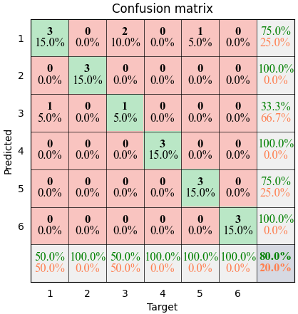
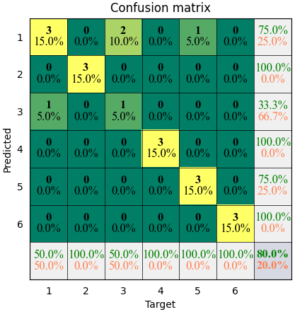
The results shown in the above figure can be obtained by the following codes.
import pyaibox as pb

T = np.array([1, 2, 3, 4, 5, 6, 1, 2, 3, 4, 5, 6, 1, 2, 3, 4, 5, 6, 1, 5])
P = np.array([1, 2, 3, 4, 1, 6, 3, 2, 1, 4, 5, 6, 1, 2, 1, 4, 5, 6, 1, 5])

C = pb.confusion(P, T, cmpmode='@')

plt = pb.plot_confusion(C, cmap=None)
plt = pb.plot_confusion(C, cmap='summer')
plt.show()
pyaibox.evaluation.contrast module
- pyaibox.evaluation.contrast.contrast(X, caxis=None, axis=None, mode='way1', reduction='mean')
Compute contrast of an complex image
'way1'is defined as follows, see [1]:\[C = \frac{\sqrt{{\rm E}\left(|I|^2 - {\rm E}(|I|^2)\right)^2}}{{\rm E}(|I|^2)} \]'way2'is defined as follows, see [2]:\[C = \frac{{\rm E}(|I|^2)}{\left({\rm E}(|I|)\right)^2} \][1] Efficient Nonparametric ISAR Autofocus Algorithm Based on Contrast Maximization and Newton [2] section 13.4.1 in “Ian G. Cumming’s SAR book”
- Parameters
X (numpy ndarray) – The image array.
caxis (int or None) – If
Xis complex-valued,caxisis ignored. IfXis real-valued andcaxisis integer thenXwill be treated as complex-valued, in this case,caxisspecifies the complex axis; otherwise (None),Xwill be treated as real-valuedaxis (int or None) – The dimension axis (
caxisis not included) for computing contrast. The default isNone, which means all.mode (str, optional) –
'way1'or'way2'reduction (str, optional) – The operation in batch dim,
None,'mean'or'sum'(the default is'mean')
- Returns
C – The contrast value of input.
- Return type
scalar or numpy array
Examples
np.random.seed(2020)
X = np.random.randn(5, 2, 3, 4)

# real
C1 = contrast(X, caxis=None, axis=(-2, -1), mode='way1', reduction=None)
C2 = contrast(X, caxis=None, axis=(-2, -1), mode='way1', reduction='sum')
C3 = contrast(X, caxis=None, axis=(-2, -1), mode='way1', reduction='mean')
print(C1, C2, C3)

# complex in real format
C1 = contrast(X, caxis=1, axis=(-2, -1), mode='way1', reduction=None)
C2 = contrast(X, caxis=1, axis=(-2, -1), mode='way1', reduction='sum')
C3 = contrast(X, caxis=1, axis=(-2, -1), mode='way1', reduction='mean')
print(C1, C2, C3)

# complex in complex format
X = X[:, 0, ...] + 1j * X[:, 1, ...]
C1 = contrast(X, caxis=None, axis=(-2, -1), mode='way1', reduction=None)
C2 = contrast(X, caxis=None, axis=(-2, -1), mode='way1', reduction='sum')
C3 = contrast(X, caxis=None, axis=(-2, -1), mode='way1', reduction='mean')
print(C1, C2, C3)

# ---output
[[1.07323512 1.39704055]
[0.96033633 1.35878254]
[1.57174342 1.42973702]
[1.37236497 1.2351262 ]
[1.06519696 1.4606771 ]] 12.924240207170865 1.2924240207170865
[0.86507341 1.03834259 1.00448054 0.89381925 1.20616657] 5.007882367336851 1.0015764734673702
[0.86507341 1.03834259 1.00448054 0.89381925 1.20616657] 5.007882367336851 1.0015764734673702
pyaibox.evaluation.detection_voc module
- pyaibox.evaluation.detection_voc.bbox_iou(bbox_a, bbox_b)
Calculate the Intersection of Unions (IoUs) between bounding boxes.
IoU is calculated as a ratio of area of the intersection and area of the union. This function accepts both
numpy.ndarrayandcupy.ndarrayas inputs. Please note that bothbbox_aandbbox_bneed to be same type. The output is same type as the type of the inputs.- Parameters
bbox_a (array) – An array whose shape is \((N, 4)\). \(N\) is the number of bounding boxes. The dtype should be
numpy.float32.bbox_b (array) – An array similar to
bbox_a, whose shape is \((K, 4)\). The dtype should benumpy.float32.
- Returns
array An array whose shape is \((N, K)\). An element at index \((n, k)\) contains IoUs between \(n\) th bounding box in
bbox_aand \(k\) th bounding box inbbox_b.
- pyaibox.evaluation.detection_voc.calc_detection_voc_ap(prec, rec, use_07_metric=False)
Calculate average precisions based on evaluation code of PASCAL VOC.
This function calculates average precisions from given precisions and recalls. The code is based on the evaluation code used in PASCAL VOC Challenge.
- Parameters
prec (list of numpy.array) – A list of arrays.
prec[l]indicates precision for class \(l\). Ifprec[l]isNone, this function returnsnumpy.nanfor class \(l\).rec (list of numpy.array) – A list of arrays.
rec[l]indicates recall for class \(l\). Ifrec[l]isNone, this function returnsnumpy.nanfor class \(l\).use_07_metric (bool) – Whether to use PASCAL VOC 2007 evaluation metric for calculating average precision. The default value is
False.
- Returns
This function returns an array of average precisions. The \(l\)-th value corresponds to the average precision for class \(l\). If
prec[l]orrec[l]isNone, the corresponding value is set tonumpy.nan.- Return type
ndarray
- pyaibox.evaluation.detection_voc.calc_detection_voc_prec_rec(pred_bboxes, pred_labels, pred_scores, gt_bboxes, gt_labels, gt_difficults=None, iou_thresh=0.5)
Calculate precision and recall based on evaluation code of PASCAL VOC.
This function calculates precision and recall of predicted bounding boxes obtained from a dataset which has \(N\) images. The code is based on the evaluation code used in PASCAL VOC Challenge.
- Parameters
pred_bboxes (iterable of numpy.ndarray) – An iterable of \(N\) sets of bounding boxes. Its index corresponds to an index for the base dataset. Each element of
pred_bboxesis a set of coordinates of bounding boxes. This is an array whose shape is \((R, 4)\), where \(R\) corresponds to the number of bounding boxes, which may vary among boxes. The second axis corresponds to \(y_{min}, x_{min}, y_{max}, x_{max}\) of a bounding box.pred_labels (iterable of numpy.ndarray) – An iterable of labels. Similar to
pred_bboxes, its index corresponds to an index for the base dataset. Its length is \(N\).pred_scores (iterable of numpy.ndarray) – An iterable of confidence scores for predicted bounding boxes. Similar to
pred_bboxes, its index corresponds to an index for the base dataset. Its length is \(N\).gt_bboxes (iterable of numpy.ndarray) – An iterable of ground truth bounding boxes whose length is \(N\). An element of
gt_bboxesis a bounding box whose shape is \((R, 4)\). Note that the number of bounding boxes in each image does not need to be same as the number of corresponding predicted boxes.gt_labels (iterable of numpy.ndarray) – An iterable of ground truth labels which are organized similarly to
gt_bboxes.gt_difficults (iterable of numpy.ndarray) – An iterable of boolean arrays which is organized similarly to
gt_bboxes. This tells whether the corresponding ground truth bounding box is difficult or not. By default, this isNone. In that case, this function considers all bounding boxes to be not difficult.iou_thresh (float) – A prediction is correct if its Intersection over Union with the ground truth is above this value..
- Returns
This function returns two lists:
precandrec.prec: A list of arrays.prec[l]is precisionfor class \(l\). If class \(l\) does not exist in either
pred_labelsorgt_labels,prec[l]is set toNone.
rec: A list of arrays.rec[l]is recallfor class \(l\). If class \(l\) that is not marked as difficult does not exist in
gt_labels,rec[l]is set toNone.
- Return type
tuple of two lists
- pyaibox.evaluation.detection_voc.eval_detection_voc(pred_bboxes, pred_labels, pred_scores, gt_bboxes, gt_labels, gt_difficults=None, iou_thresh=0.5, use_07_metric=False)
Calculate average precisions based on evaluation code of PASCAL VOC.
This function evaluates predicted bounding boxes obtained from a dataset which has \(N\) images by using average precision for each class. The code is based on the evaluation code used in PASCAL VOC Challenge.
- Parameters
pred_bboxes (iterable of numpy.ndarray) – An iterable of \(N\) sets of bounding boxes. Its index corresponds to an index for the base dataset. Each element of
pred_bboxesis a set of coordinates of bounding boxes. This is an array whose shape is \((R, 4)\), where \(R\) corresponds to the number of bounding boxes, which may vary among boxes. The second axis corresponds to \(y_{min}, x_{min}, y_{max}, x_{max}\) of a bounding box.pred_labels (iterable of numpy.ndarray) – An iterable of labels. Similar to
pred_bboxes, its index corresponds to an index for the base dataset. Its length is \(N\).pred_scores (iterable of numpy.ndarray) – An iterable of confidence scores for predicted bounding boxes. Similar to
pred_bboxes, its index corresponds to an index for the base dataset. Its length is \(N\).gt_bboxes (iterable of numpy.ndarray) – An iterable of ground truth bounding boxes whose length is \(N\). An element of
gt_bboxesis a bounding box whose shape is \((R, 4)\). Note that the number of bounding boxes in each image does not need to be same as the number of corresponding predicted boxes.gt_labels (iterable of numpy.ndarray) – An iterable of ground truth labels which are organized similarly to
gt_bboxes.gt_difficults (iterable of numpy.ndarray) – An iterable of boolean arrays which is organized similarly to
gt_bboxes. This tells whether the corresponding ground truth bounding box is difficult or not. By default, this isNone. In that case, this function considers all bounding boxes to be not difficult.iou_thresh (float) – A prediction is correct if its Intersection over Union with the ground truth is above this value.
use_07_metric (bool) – Whether to use PASCAL VOC 2007 evaluation metric for calculating average precision. The default value is
False.
- Returns
The keys, value-types and the description of the values are listed below.
- ap (ndarray): An array of average precisions.
The \(l\)-th value corresponds to the average precision for class \(l\). If class \(l\) does not exist in either
pred_labelsorgt_labels, the corresponding value is set tonumpy.nan.
map (float): The average of Average Precisions over classes.
- Return type
pyaibox.evaluation.entropy module
- pyaibox.evaluation.entropy.entropy(X, caxis=None, axis=None, mode='shannon', reduction='mean')
compute the entropy of the inputs
\[{\rm ENT} = -\sum_{n=0}^N p_i{\rm log}_2 p_n \]where \(N\) is the number of pixels, \(p_n=\frac{|X_n|^2}{\sum_{n=0}^N|X_n|^2}\).
- Parameters
X (numpy array) – The complex or real inputs, for complex inputs, both complex and real representations are surpported.
caxis (int or None) – If
Xis complex-valued,caxisis ignored. IfXis real-valued andcaxisis integer thenXwill be treated as complex-valued, in this case,caxisspecifies the complex axis; otherwise (None),Xwill be treated as real-valuedaxis (int or None) – The dimension axis (
caxisis not included) for computing entropy. The default isNone, which means all.mode (str, optional) – The entropy mode:
'shannon'or'natural'(the default is ‘shannon’)reduction (str, optional) – The operation in batch dim,
None,'mean'or'sum'(the default is'mean')
- Returns
S – The entropy of the inputs.
- Return type
scalar or numpy array
Examples
np.random.seed(2020)
X = np.random.randn(5, 2, 3, 4)

# real
S1 = entropy(X, caxis=None, axis=(-2, -1), mode='shannon', reduction=None)
S2 = entropy(X, caxis=None, axis=(-2, -1), mode='shannon', reduction='sum')
S3 = entropy(X, caxis=None, axis=(-2, -1), mode='shannon', reduction='mean')
print(S1, S2, S3)

# complex in real format
S1 = entropy(X, caxis=1, axis=(-2, -1), mode='shannon', reduction=None)
S2 = entropy(X, caxis=1, axis=(-2, -1), mode='shannon', reduction='sum')
S3 = entropy(X, caxis=1, axis=(-2, -1), mode='shannon', reduction='mean')
print(S1, S2, S3)

# complex in complex format
X = X[:, 0, ...] + 1j * X[:, 1, ...]
S1 = entropy(X, caxis=None, axis=(-2, -1), mode='shannon', reduction=None)
S2 = entropy(X, caxis=None, axis=(-2, -1), mode='shannon', reduction='sum')
S3 = entropy(X, caxis=None, axis=(-2, -1), mode='shannon', reduction='mean')
print(S1, S2, S3)

# ---output
[[2.76482544 2.38657794]
[2.85232291 2.33204624]
[2.26890769 2.4308547 ]
[2.50283407 2.56037192]
[2.76608007 2.47020486]] 25.33502585795305 2.533502585795305
[3.03089227 2.84108823 2.93389666 3.00868855 2.8229912 ] 14.637556915006513 2.9275113830013026
[3.03089227 2.84108823 2.93389666 3.00868855 2.8229912 ] 14.637556915006513 2.9275113830013026
pyaibox.evaluation.error module
- pyaibox.evaluation.error.ampphaerror(orig, reco)
compute amplitude phase error
compute amplitude phase error of two complex valued matrix
- Parameters
orig (numpy array) – orignal
reco (numpy array) – reconstructed
- Returns
amperror (float) – error of amplitude
phaerror (float) – error of phase
- pyaibox.evaluation.error.mae(X, Y, caxis=None, axis=None, keepcaxis=False, reduction='mean')
computes the mean absoluted error
Both complex and real representation are supported.
\[{\rm MAE}({\bf X, Y}) = \frac{1}{N}\||{\bf X} - {\bf Y}|\| = \frac{1}{N}\sum_{i=1}^N |x_i - y_i| \]- Parameters
X (array) – original
Y (array) – reconstructed
caxis (int or None) – If
Xis complex-valued,caxisis ignored. IfXis real-valued andcaxisis integer thenXwill be treated as complex-valued, in this case,caxisspecifies the complex axis; otherwise (None),Xwill be treated as real-valuedaxis (int or None) – The dimension axis (
caxisis not included) for computing norm. The default isNone, which means all.keepcaxis (bool) – If
True, the complex dimension will be keeped. Only works whenXis complex-valued tensor but represents in real format. Default isFalse.reduction (str, optional) – The operation in batch dim,
None,'mean'or'sum'(the default is'mean')
- Returns
mean absoluted error
- Return type
scalar or array
Examples
norm = False
np.random.seed(2020)
X = np.random.randn(5, 2, 3, 4)
Y = np.random.randn(5, 2, 3, 4)

# real
C1 = mae(X, Y, caxis=None, axis=(-2, -1), reduction=None)
C2 = mae(X, Y, caxis=None, axis=(-2, -1), reduction='sum')
C3 = mae(X, Y, caxis=None, axis=(-2, -1), reduction='mean')
print(C1, C2, C3)

# complex in real format
C1 = mae(X, Y, caxis=1, axis=(-2, -1), reduction=None)
C2 = mae(X, Y, caxis=1, axis=(-2, -1), reduction='sum')
C3 = mae(X, Y, caxis=1, axis=(-2, -1), reduction='mean')
print(C1, C2, C3)

# complex in complex format
X = X[:, 0, ...] + 1j * X[:, 1, ...]
Y = Y[:, 0, ...] + 1j * Y[:, 1, ...]
C1 = mae(X, Y, caxis=None, axis=(-2, -1), reduction=None)
C2 = mae(X, Y, caxis=None, axis=(-2, -1), reduction='sum')
C3 = mae(X, Y, caxis=None, axis=(-2, -1), reduction='mean')
print(C1, C2, C3)

# ---output
[[1.06029116 1.19884877]
[0.90117091 1.13552361]
[1.23422083 0.75743914]
[1.16127965 1.42169262]
[1.25090731 1.29134222]] 11.41271620974502 1.141271620974502
[1.71298566 1.50327364 1.53328572 2.11430946 2.01435599] 8.878210471231741 1.7756420942463482
[1.71298566 1.50327364 1.53328572 2.11430946 2.01435599] 8.878210471231741 1.7756420942463482
- pyaibox.evaluation.error.mse(X, Y, caxis=None, axis=None, keepcaxis=False, reduction='mean')
computes the mean square error
Both complex and real representation are supported.
\[{\rm MSE}({\bf X, Y}) = \frac{1}{N}\|{\bf X} - {\bf Y}\|_2^2 = \frac{1}{N}\sum_{i=1}^N(|x_i - y_i|)^2 \]- Parameters
X (array) – reconstructed
Y (array) – target
caxis (int or None) – If
Xis complex-valued,caxisis ignored. IfXis real-valued andcaxisis integer thenXwill be treated as complex-valued, in this case,caxisspecifies the complex axis; otherwise (None),Xwill be treated as real-valuedaxis (int or None) – The dimension axis (
caxisis not included) for computing norm. The default isNone, which means all.keepcaxis (bool) – If
True, the complex dimension will be keeped. Only works whenXis complex-valued tensor but represents in real format. Default isFalse.reduction (str, optional) – The operation in batch dim,
None,'mean'or'sum'(the default is'mean')
- Returns
mean square error
- Return type
scalar or array
Examples
norm = False
np.random.seed(2020)
X = np.random.randn(5, 2, 3, 4)
Y = np.random.randn(5, 2, 3, 4)

# real
C1 = mse(X, Y, caxis=None, axis=(-2, -1), reduction=None)
C2 = mse(X, Y, caxis=None, axis=(-2, -1), reduction='sum')
C3 = mse(X, Y, caxis=None, axis=(-2, -1), reduction='mean')
print(C1, C2, C3)

# complex in real format
C1 = mse(X, Y, caxis=1, axis=(-2, -1), reduction=None)
C2 = mse(X, Y, caxis=1, axis=(-2, -1), reduction='sum')
C3 = mse(X, Y, caxis=1, axis=(-2, -1), reduction='mean')
print(C1, C2, C3)

# complex in complex format
X = X[:, 0, ...] + 1j * X[:, 1, ...]
Y = Y[:, 0, ...] + 1j * Y[:, 1, ...]
C1 = mse(X, Y, caxis=None, axis=(-2, -1), reduction=None)
C2 = mse(X, Y, caxis=None, axis=(-2, -1), reduction='sum')
C3 = mse(X, Y, caxis=None, axis=(-2, -1), reduction='mean')
print(C1, C2, C3)

# ---output
[[1.57602573 2.32844311]
[1.07232374 2.36118382]
[2.1841515  0.79002805]
[2.43036295 3.18413899]
[2.31107373 2.73990485]] 20.977636476183186 2.0977636476183186
[3.90446884 3.43350757 2.97417955 5.61450194 5.05097858] 20.977636476183186 4.195527295236637
[3.90446884 3.43350757 2.97417955 5.61450194 5.05097858] 20.977636476183186 4.195527295236637
- pyaibox.evaluation.error.nmae(X, Y, caxis=None, axis=None, keepcaxis=False, reduction='mean')
computes the normalized mean absoluted error
Both complex and real representation are supported.
\[{\rm NMAE}({\bf X, Y}) = \frac{\frac{1}{N}\||{\bf X} - {\bf Y}|\|}{\||{\bf Y}|\|} \]- Parameters
X (array) – original
Y (array) – reconstructed
caxis (int or None) – If
Xis complex-valued,caxisis ignored. IfXis real-valued andcaxisis integer thenXwill be treated as complex-valued, in this case,caxisspecifies the complex axis; otherwise (None),Xwill be treated as real-valuedaxis (int or None) – The dimension axis (
caxisis not included) for computing norm. The default isNone, which means all.keepcaxis (bool) – If
True, the complex dimension will be keeped. Only works whenXis complex-valued tensor but represents in real format. Default isFalse.reduction (str, optional) – The operation in batch dim,
None,'mean'or'sum'(the default is'mean')
- Returns
mean absoluted error
- Return type
scalar or array
Examples
np.random.seed(2020)
X = np.random.randn(5, 2, 3, 4)
Y = np.random.randn(5, 2, 3, 4)

# real
C1 = nmae(X, Y, caxis=None, axis=(-2, -1), reduction=None)
C2 = nmae(X, Y, caxis=None, axis=(-2, -1), reduction='sum')
C3 = nmae(X, Y, caxis=None, axis=(-2, -1), reduction='mean')
print(C1, C2, C3)

# complex in real format
C1 = nmae(X, Y, caxis=1, axis=(-2, -1), reduction=None)
C2 = nmae(X, Y, caxis=1, axis=(-2, -1), reduction='sum')
C3 = nmae(X, Y, caxis=1, axis=(-2, -1), reduction='mean')
print(C1, C2, C3)

# complex in complex format
X = X[:, 0, ...] + 1j * X[:, 1, ...]
Y = Y[:, 0, ...] + 1j * Y[:, 1, ...]
C1 = nmae(X, Y, caxis=None, axis=(-2, -1), reduction=None)
C2 = nmae(X, Y, caxis=None, axis=(-2, -1), reduction='sum')
C3 = nmae(X, Y, caxis=None, axis=(-2, -1), reduction='mean')
print(C1, C2, C3)
- pyaibox.evaluation.error.nmse(X, Y, caxis=None, axis=None, keepcaxis=False, reduction='mean')
computes the normalized mean square error
Both complex and real representation are supported.
\[{\rm NMSE}({\bf X, Y}) = \frac{\frac{1}{N}\|{\bf X} - {\bf Y}\|_2^2}{\|{\bf Y}\|_2^2}= \frac{\frac{1}{N}\sum_{i=1}^N(|x_i - y_i|)^2}{\sum_{i=1}^N(|y_i|)^2} \]- Parameters
X (array) – reconstructed
Y (array) – target
caxis (int or None) – If
Xis complex-valued,caxisis ignored. IfXis real-valued andcaxisis integer thenXwill be treated as complex-valued, in this case,caxisspecifies the complex axis; otherwise (None),Xwill be treated as real-valuedaxis (int or None) – The dimension axis (
caxisis not included) for computing norm. The default isNone, which means all.keepcaxis (bool) – If
True, the complex dimension will be keeped. Only works whenXis complex-valued tensor but represents in real format. Default isFalse.reduction (str, optional) – The operation in batch dim,
None,'mean'or'sum'(the default is'mean')
- Returns
mean square error
- Return type
scalar or array
Examples
np.random.seed(2020)
X = np.random.randn(5, 2, 3, 4)
Y = np.random.randn(5, 2, 3, 4)

# real
C1 = nmse(X, Y, caxis=None, axis=(-2, -1), reduction=None)
C2 = nmse(X, Y, caxis=None, axis=(-2, -1), reduction='sum')
C3 = nmse(X, Y, caxis=None, axis=(-2, -1), reduction='mean')
print(C1, C2, C3)

# complex in real format
C1 = nmse(X, Y, caxis=1, axis=(-2, -1), reduction=None)
C2 = nmse(X, Y, caxis=1, axis=(-2, -1), reduction='sum')
C3 = nmse(X, Y, caxis=1, axis=(-2, -1), reduction='mean')
print(C1, C2, C3)

# complex in complex format
X = X[:, 0, ...] + 1j * X[:, 1, ...]
Y = Y[:, 0, ...] + 1j * Y[:, 1, ...]
C1 = nmse(X, Y, caxis=None, axis=(-2, -1), reduction=None)
C2 = nmse(X, Y, caxis=None, axis=(-2, -1), reduction='sum')
C3 = nmse(X, Y, caxis=None, axis=(-2, -1), reduction='mean')
print(C1, C2, C3)
- pyaibox.evaluation.error.nsae(X, Y, caxis=None, axis=None, keepcaxis=False, reduction='mean')
computes the normalized sum absoluted error
Both complex and real representation are supported.
\[{\rm NSAE}({\bf X, Y}) = \frac{\||{\bf X} - {\bf Y}|\|}{\||{\bf Y}|\|} = \frac{\sum_{i=1}^N |x_i - y_i|}{\sum_{i=1}^N |y_i|} \]- Parameters
X (array) – original
Y (array) – reconstructed
caxis (int or None) – If
Xis complex-valued,caxisis ignored. IfXis real-valued andcaxisis integer thenXwill be treated as complex-valued, in this case,caxisspecifies the complex axis; otherwise (None),Xwill be treated as real-valuedaxis (int or None) – The dimension axis (
caxisis not included) for computing norm. The default isNone, which means all.keepcaxis (bool) – If
True, the complex dimension will be keeped. Only works whenXis complex-valued tensor but represents in real format. Default isFalse.reduction (str, optional) – The operation in batch dim,
None,'mean'or'sum'(the default is'mean')
- Returns
sum absoluted error
- Return type
scalar or array
Examples
np.random.seed(2020)
X = np.random.randn(5, 2, 3, 4)
Y = np.random.randn(5, 2, 3, 4)

# real
C1 = nsae(X, Y, caxis=None, axis=(-2, -1), reduction=None)
C2 = nsae(X, Y, caxis=None, axis=(-2, -1), reduction='sum')
C3 = nsae(X, Y, caxis=None, axis=(-2, -1), reduction='mean')
print(C1, C2, C3)

# complex in real format
C1 = nsae(X, Y, caxis=1, axis=(-2, -1), reduction=None)
C2 = nsae(X, Y, caxis=1, axis=(-2, -1), reduction='sum')
C3 = nsae(X, Y, caxis=1, axis=(-2, -1), reduction='mean')
print(C1, C2, C3)

# complex in complex format
X = X[:, 0, ...] + 1j * X[:, 1, ...]
Y = Y[:, 0, ...] + 1j * Y[:, 1, ...]
C1 = nsae(X, Y, caxis=None, axis=(-2, -1), reduction=None)
C2 = nsae(X, Y, caxis=None, axis=(-2, -1), reduction='sum')
C3 = nsae(X, Y, caxis=None, axis=(-2, -1), reduction='mean')
print(C1, C2, C3)
- pyaibox.evaluation.error.nsse(X, Y, caxis=None, axis=None, keepcaxis=False, reduction='mean')
computes the normalized sum square error
Both complex and real representation are supported.
\[{\rm NSSE}({\bf X, Y}) = \frac{\|{\bf X} - {\bf Y}\|_2^2}{\|{\bf Y}\|_2^2} = \frac{\sum_{i=1}^N(|x_i - y_i|)^2}{\sum_{i=1}^N(|y_i|)^2} \]- Parameters
X (array) – reconstructed
Y (array) – target
caxis (int or None) – If
Xis complex-valued,caxisis ignored. IfXis real-valued andcaxisis integer thenXwill be treated as complex-valued, in this case,caxisspecifies the complex axis; otherwise (None),Xwill be treated as real-valuedaxis (int or None) – The dimension axis (
caxisis not included) for computing norm. The default isNone, which means all.keepcaxis (bool) – If
True, the complex dimension will be keeped. Only works whenXis complex-valued tensor but represents in real format. Default isFalse.reduction (str, optional) – The operation in batch dim,
None,'mean'or'sum'(the default is'mean')
- Returns
sum square error
- Return type
scalar or array
Examples
np.random.seed(2020)
X = np.random.randn(5, 2, 3, 4)
Y = np.random.randn(5, 2, 3, 4)

# real
C1 = sse(X, Y, caxis=None, axis=(-2, -1), reduction=None)
C2 = sse(X, Y, caxis=None, axis=(-2, -1), reduction='sum')
C3 = sse(X, Y, caxis=None, axis=(-2, -1), reduction='mean')
print(C1, C2, C3)

# complex in real format
C1 = sse(X, Y, caxis=1, axis=(-2, -1), reduction=None)
C2 = sse(X, Y, caxis=1, axis=(-2, -1), reduction='sum')
C3 = sse(X, Y, caxis=1, axis=(-2, -1), reduction='mean')
print(C1, C2, C3)

# complex in complex format
X = X[:, 0, ...] + 1j * X[:, 1, ...]
Y = Y[:, 0, ...] + 1j * Y[:, 1, ...]
C1 = sse(X, Y, caxis=None, axis=(-2, -1), reduction=None)
C2 = sse(X, Y, caxis=None, axis=(-2, -1), reduction='sum')
C3 = sse(X, Y, caxis=None, axis=(-2, -1), reduction='mean')
print(C1, C2, C3)
- pyaibox.evaluation.error.sae(X, Y, caxis=None, axis=None, keepcaxis=False, reduction='mean')
computes the sum absoluted error
Both complex and real representation are supported.
\[{\rm SAE}({\bf X, Y}) = \||{\bf X} - {\bf Y}|\| = \sum_{i=1}^N |x_i - y_i| \]- Parameters
X (array) – original
Y (array) – reconstructed
caxis (int or None) – If
Xis complex-valued,caxisis ignored. IfXis real-valued andcaxisis integer thenXwill be treated as complex-valued, in this case,caxisspecifies the complex axis; otherwise (None),Xwill be treated as real-valuedaxis (int or None) – The dimension axis (
caxisis not included) for computing norm. The default isNone, which means all.keepcaxis (bool) – If
True, the complex dimension will be keeped. Only works whenXis complex-valued tensor but represents in real format. Default isFalse.reduction (str, optional) – The operation in batch dim,
None,'mean'or'sum'(the default is'mean')
- Returns
sum absoluted error
- Return type
scalar or array
Examples
norm = False
np.random.seed(2020)
X = np.random.randn(5, 2, 3, 4)
Y = np.random.randn(5, 2, 3, 4)

# real
C1 = sae(X, Y, caxis=None, axis=(-2, -1), reduction=None)
C2 = sae(X, Y, caxis=None, axis=(-2, -1), reduction='sum')
C3 = sae(X, Y, caxis=None, axis=(-2, -1), reduction='mean')
print(C1, C2, C3)

# complex in real format
C1 = sae(X, Y, caxis=1, axis=(-2, -1), reduction=None)
C2 = sae(X, Y, caxis=1, axis=(-2, -1), reduction='sum')
C3 = sae(X, Y, caxis=1, axis=(-2, -1), reduction='mean')
print(C1, C2, C3)

# complex in complex format
X = X[:, 0, ...] + 1j * X[:, 1, ...]
Y = Y[:, 0, ...] + 1j * Y[:, 1, ...]
C1 = sae(X, Y, caxis=None, axis=(-2, -1), reduction=None)
C2 = sae(X, Y, caxis=None, axis=(-2, -1), reduction='sum')
C3 = sae(X, Y, caxis=None, axis=(-2, -1), reduction='mean')
print(C1, C2, C3)

# ---output
[[12.72349388 14.3861852 ]
[10.81405096 13.62628335]
[14.81065     9.08926963]
[13.93535577 17.0603114 ]
[15.0108877  15.49610662]] 136.95259451694022 13.695259451694023
[20.55582795 18.03928365 18.39942858 25.37171356 24.17227192] 106.53852565478087 21.307705130956172
[20.55582795 18.03928365 18.39942858 25.37171356 24.17227192] 106.5385256547809 21.30770513095618
- pyaibox.evaluation.error.sse(X, Y, caxis=None, axis=None, keepcaxis=False, reduction='mean')
computes the sum square error
Both complex and real representation are supported.
\[{\rm SSE}({\bf X, Y}) = \|{\bf X} - {\bf Y}\|_2^2 = \sum_{i=1}^N(|x_i - y_i|)^2 \]- Parameters
X (array) – reconstructed
Y (array) – target
caxis (int or None) – If
Xis complex-valued,caxisis ignored. IfXis real-valued andcaxisis integer thenXwill be treated as complex-valued, in this case,caxisspecifies the complex axis; otherwise (None),Xwill be treated as real-valuedaxis (int or None) – The dimension axis (
caxisis not included) for computing norm. The default isNone, which means all.keepcaxis (bool) – If
True, the complex dimension will be keeped. Only works whenXis complex-valued tensor but represents in real format. Default isFalse.reduction (str, optional) – The operation in batch dim,
None,'mean'or'sum'(the default is'mean')
- Returns
sum square error
- Return type
scalar or array
Examples
norm = False
np.random.seed(2020)
X = np.random.randn(5, 2, 3, 4)
Y = np.random.randn(5, 2, 3, 4)

# real
C1 = sse(X, Y, caxis=None, axis=(-2, -1), reduction=None)
C2 = sse(X, Y, caxis=None, axis=(-2, -1), reduction='sum')
C3 = sse(X, Y, caxis=None, axis=(-2, -1), reduction='mean')
print(C1, C2, C3)

# complex in real format
C1 = sse(X, Y, caxis=1, axis=(-2, -1), reduction=None)
C2 = sse(X, Y, caxis=1, axis=(-2, -1), reduction='sum')
C3 = sse(X, Y, caxis=1, axis=(-2, -1), reduction='mean')
print(C1, C2, C3)

# complex in complex format
X = X[:, 0, ...] + 1j * X[:, 1, ...]
Y = Y[:, 0, ...] + 1j * Y[:, 1, ...]
C1 = sse(X, Y, caxis=None, axis=(-2, -1), reduction=None)
C2 = sse(X, Y, caxis=None, axis=(-2, -1), reduction='sum')
C3 = sse(X, Y, caxis=None, axis=(-2, -1), reduction='mean')
print(C1, C2, C3)

# ---output
[[18.91230872 27.94131733]
[12.86788492 28.33420589]
[26.209818    9.48033663]
[29.16435541 38.20966786]
[27.73288477 32.87885818]] 251.73163771419823 25.173163771419823
[46.85362605 41.20209081 35.69015462 67.37402327 60.61174295] 251.73163771419823 50.346327542839646
[46.85362605 41.20209081 35.69015462 67.37402327 60.61174295] 251.73163771419823 50.346327542839646
pyaibox.evaluation.norm module
- pyaibox.evaluation.norm.fnorm(X, caxis=None, axis=None, reduction='mean')
obtain the f-norm of a array
Both complex and real representation are supported.
\[{\rm fnorm}({\bf X}) = \|{\bf X}\|_2 = \left(\sum_{x_i\in {\bf X}}|x_i|^2\right)^{\frac{1}{2}} = \left(\sum_{x_i\in {\bf X}}(u_i^2 + v_i^2)\right)^{\frac{1}{2}} \]where, \(u, v\) are the real and imaginary part of \(x\), respectively.
- Parameters
X (array) – input
caxis (int or None) – If
Xis complex-valued,caxisis ignored. IfXis real-valued andcaxisis integer thenXwill be treated as complex-valued, in this case,caxisspecifies the complex axis; otherwise (None),Xwill be treated as real-valuedaxis (int or None) – The dimension axis (
caxisis not included) for computing norm. The default isNone, which means all.reduction (str, optional) – The operation in batch dim,
None,'mean'or'sum'(the default is'mean')
- Returns
the inputs’s f-norm.
- Return type
array
Examples
np.random.seed(2020)
X = np.random.randn(5, 2, 3, 4)

# real
C1 = fnorm(X, caxis=None, axis=(-2, -1), reduction=None)
C2 = fnorm(X, caxis=None, axis=(-2, -1), reduction='sum')
C3 = fnorm(X, caxis=None, axis=(-2, -1), reduction='mean')
print(C1, C2, C3)

# complex in real format
C1 = fnorm(X, caxis=1, axis=(-2, -1), reduction=None)
C2 = fnorm(X, caxis=1, axis=(-2, -1), reduction='sum')
C3 = fnorm(X, caxis=1, axis=(-2, -1), reduction='mean')
print(C1, C2, C3)

# complex in complex format
X = X[:, 0, ...] + 1j * X[:, 1, ...]
C1 = fnorm(X, caxis=None, axis=(-2, -1), reduction=None)
C2 = fnorm(X, caxis=None, axis=(-2, -1), reduction='sum')
C3 = fnorm(X, caxis=None, axis=(-2, -1), reduction='mean')
print(C1, C2, C3)

# ---output
---norm
[[3.18214671 3.28727232]
[3.52423801 3.45821738]
[3.07757733 3.23720035]
[2.45488229 3.98372024]
[2.23480914 3.73551246]] 32.1755762254205 3.21755762254205
[4.57517398 4.93756225 4.46664844 4.67936684 4.35297889] 23.011730410021634 4.602346082004327
[4.57517398 4.93756225 4.46664844 4.67936684 4.35297889] 23.011730410021634 4.602346082004327
- pyaibox.evaluation.norm.pnorm(X, caxis=None, axis=None, p=2, reduction='mean')
obtain the p-norm of a array
Both complex and real representation are supported.
\[{\rm pnorm}({\bf X}) = \|{\bf X}\|_p = \left(\sum_{x_i\in {\bf X}}|x_i|^p\right)^{\frac{1}{p}} = \left(\sum_{x_i\in {\bf X}}\sqrt{u_i^2+v^2}^p\right)^{\frac{1}{p}} \]where, \(u, v\) are the real and imaginary part of \(x\), respectively.
- Parameters
X (array) – input
caxis (int or None) – If
Xis complex-valued,caxisis ignored. IfXis real-valued andcaxisis integer thenXwill be treated as complex-valued, in this case,caxisspecifies the complex axis; otherwise (None),Xwill be treated as real-valuedaxis (int or None) – The dimension axis (
caxisis not included) for computing norm. The default isNone, which means all.p (int) – Specifies the power. The default is 2.
reduction (str, optional) – The operation in batch dim,
None,'mean'or'sum'(the default is'mean')
- Returns
the inputs’s p-norm.
- Return type
array
Examples
np.random.seed(2020)
X = np.random.randn(5, 2, 3, 4)

# real
C1 = pnorm(X, caxis=None, axis=(-2, -1), reduction=None)
C2 = pnorm(X, caxis=None, axis=(-2, -1), reduction='sum')
C3 = pnorm(X, caxis=None, axis=(-2, -1), reduction='mean')
print(C1, C2, C3)

# complex in real format
C1 = pnorm(X, caxis=1, axis=(-2, -1), reduction=None)
C2 = pnorm(X, caxis=1, axis=(-2, -1), reduction='sum')
C3 = pnorm(X, caxis=1, axis=(-2, -1), reduction='mean')
print(C1, C2, C3)

# complex in complex format
X = X[:, 0, ...] + 1j * X[:, 1, ...]
C1 = pnorm(X, caxis=None, axis=(-2, -1), reduction=None)
C2 = pnorm(X, caxis=None, axis=(-2, -1), reduction='sum')
C3 = pnorm(X, caxis=None, axis=(-2, -1), reduction='mean')
print(C1, C2, C3)

# ---output
---pnorm
[[3.18214671 3.28727232]
[3.52423801 3.45821738]
[3.07757733 3.23720035]
[2.45488229 3.98372024]
[2.23480914 3.73551246]] 32.1755762254205 3.21755762254205
[4.57517398 4.93756225 4.46664844 4.67936684 4.35297889] 23.011730410021634 4.602346082004327
[4.57517398 4.93756225 4.46664844 4.67936684 4.35297889] 23.011730410021634 4.602346082004327
pyaibox.evaluation.snrs module
- pyaibox.evaluation.snrs.psnr(P, G, vpeak=None, **kwargs)
Peak Signal-to-Noise Ratio
The Peak Signal-to-Noise Ratio (PSNR) is expressed as
\[{\rm psnrv} = 10 \log10(\frac{V_{\rm peak}^2}{\rm MSE}) \]For float data, \(V_{\rm peak} = 1\);
For interges, \(V_{\rm peak} = 2^{\rm nbits}\), e.g. uint8: 255, uint16: 65535 …
- Parameters
P (array_like) – The data to be compared. For image, it’s the reconstructed image.
G (array_like) – Reference data array. For image, it’s the original image.
vpeak (float, int or None, optional) – The peak value. If None, computes automaticly.
caxis (None or int, optional) – If
PandGare complex-valued but represented in real format,caxisorcdimshould be specified. If not, it’s set toNone, which meansPandGare real-valued or complex-valued in complex format.keepcaxis (int or None, optional) – keep the complex dimension?
axis (int or None, optional) – Specifies the dimensions for computing SNR, if not specified, it’s set to
None, which means all the dimensions.reduction (str, optional) – The reduce operation in batch dimension. Supported are
'mean','sum'orNone. If not specified, it is set toNone.
- Returns
psnrv – Peak Signal to Noise Ratio value.
- Return type
Examples
import torch as th
import pyaibox as pb

pb.setseed(seed=2020, target='numpy')
P = 255. * np.random.rand(5, 2, 3, 4)
G = 255. * np.random.rand(5, 2, 3, 4)
snrv = psnr(P, G, caxis=1, dim=(2, 3), keepcaxis=True)
print(snrv)
snrv = psnr(P, G, caxis=1, dim=(2, 3), keepcaxis=True, reduction='mean')
print(snrv)
P = pb.r2c(P, caxis=1, keepcaxis=False)
G = pb.r2c(G, caxis=1, keepcaxis=False)
snrv = psnr(P, G, caxis=None, dim=(1, 2), reduction='mean')
print(snrv)

# ---output
[[4.93636105]
[5.1314932 ]
[4.65173472]
[5.05826362]
[5.20860623]]
4.997291765071102
4.997291765071102
- pyaibox.evaluation.snrs.snr(x, n=None, **kwargs)
computes signal-to-noise ratio
\[{\rm SNR} = 10*{\rm log10}(\frac{P_x}{P_n}) \]where, \(P_x, P_n\) are the power summary of the signal and noise:
\[P_x = \sum_{i=1}^N |x_i|^2 \\ P_n = \sum_{i=1}^N |n_i|^2 \]snr(x, n)equals to matlab’ssnr(x, n)- Parameters
x (tensor) – The pure signal data.
n (ndarray, tensor) – The noise data.
caxis (None or int, optional) – If
xandnare complex-valued but represented in real format,caxisorcdimshould be specified. If not, it’s set toNone, which meansxandnare real-valued or complex-valued in complex format.keepcaxis (int or None, optional) – keep the complex dimension?
axis (int or None, optional) – Specifies the dimensions for computing SNR, if not specified, it’s set to
None, which means all the dimensions.reduction (str, optional) – The reduce operation in batch dimension. Supported are
'mean','sum'orNone. If not specified, it is set toNone.
- Returns
The SNRs.
- Return type
scalar
Examples
import torch as th
import pyaibox as pb

pb.setseed(seed=2020, target='numpy')
x = 10 * th.randn(5, 2, 3, 4)
n = th.randn(5, 2, 3, 4)
snrv = snr(x, n, caxis=1, axis=(2, 3), keepcaxis=True)
print(snrv)
snrv = snr(x, n, caxis=1, axis=(2, 3), keepcaxis=True, reduction='mean')
print(snrv)
x = pb.r2c(x, caxis=1, keepcaxis=False)
n = pb.r2c(n, caxis=1, keepcaxis=False)
snrv = snr(x, n, caxis=None, axis=(1, 2), reduction='mean')
print(snrv)

---output
[[19.36533589]
[20.09428302]
[19.29255523]
[19.81755215]
[17.88677726]]
19.291300709856387
19.291300709856387