torchlib.optim package
Submodules
torchlib.optim.learning_rate module
- class torchlib.optim.learning_rate.LrFinder(device='cpu', plotdir=None, logf=None)
Bases:
object- find(dataloader, model, optimizer, criterion, nin=1, nout=1, nbgc=1, lr_init=1e-08, lr_final=100.0, beta=0.98, gamma=4.0)
Find learning rate
Find learning rate, see How Do You Find A Good Learning Rate .
During traing, two types losses are computed
The average loss is:
\[\rm{avg\_loss}_i=\beta * \rm{avg\_loss}_{i-1}+(1-\beta) * \rm{loss}_i \]The smoothed loss is:
\[\rm{smt\_loss }_{i}=\frac{\rm{avg\_loss}_{i}}{1-\beta^{i+1}} \]If \(i > 1\) and \(\rm{smt\_loss} > \gamma * \rm{best\_loss}\), stop.
If \(\rm{smt\_loss} < \rm{best\_loss}\) or \(i = 1\), let \(\rm{best\_loss} = \rm{smt\_loss}\).
- Parameters
dataloader (DataLoader) – The dataloader that contains a dataset for training.
model (Module) – Your network module.
optimizer (Optimizer) – The optimizer such as SGD, Adam…
criterion (Loss) – The criterion/loss used for training model.
nin (int, optional) – The number of inputs of the model, the first
ninelements are inputs, the rest are targets(can be None) used for computing loss. (the default is 1)nou (int, optional) – The number of outputs of the model used for computing loss, it works only when the model has multiple outputs, i.e. the outputs is a tuple or list which has several tensor elements (>=1). the first
noutelements are used for computing loss, the rest are ignored. (the default is 1)nbgc (int, optional) – The number of batches for grad cumulation (the default is 1, which means no cumulation)
lr_init (int, optional) – The initial learning rate (the default is 1e-8)
lr_final (int, optional) – The final learning rate (the default is 1e-8)
beta (float, optional) – weight for weighted sum of loss (the default is 0.98)
gamma (float, optional) – The exploding factor \(\gamma\). (the default is 4.)
- Returns
lrs (list) – Learning rates during training.
smt_losses (list) – Smoothed losses during training.
avg_losses (list) – Average losses during training.
losses (list) – Original losses during training.
Examples
device = 'cuda:1'
# device = 'cpu'

num_epochs = 30
X = th.randn(100, 2, 3, 4)
Y = th.randn(100, 1, 3, 4)

trainds = TensorDataset(X, Y)
# trainds = TensorDataset(X)

model = th.nn.Conv2d(2, 1, 1)
model.to(device)

trainld = DataLoader(trainds, batch_size=10, shuffle=False)

criterion = th.nn.MSELoss(reduction='mean')

optimizer = th.optim.SGD(model.parameters(), lr=1e-1)

lrfinder = LrFinder(device)
# lrfinder = LrFinder(device, plotdir='./')

lrfinder.find(trainld, model, optimizer, criterion, nin=1,
              nbgc=1, lr_init=1e-8, lr_final=10., beta=0.98)

lrfinder.plot(lrmod='Linear')
lrfinder.plot(lrmod='Log')
- plot(lrmod='log', loss='smoothed')
plot the loss-lr curve
Plot the loss-learning rate curve.
- torchlib.optim.learning_rate.gammalr(x, k=2, t=2, a=1)
torchlib.optim.lr_scheduler module
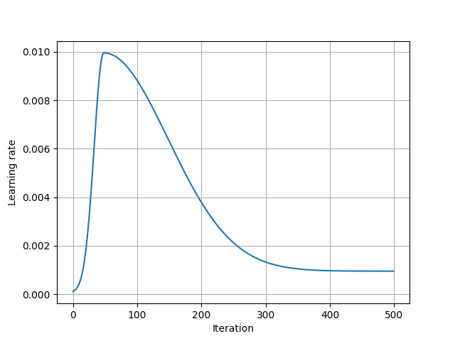
- class torchlib.optim.lr_scheduler.GaussianLR(optimizer, t_eta_max, sigma1, sigma2, eta_start=1e-06, eta_stop=1e-05, last_epoch=- 1)
Bases:
torch.optim.lr_scheduler._LRSchedulerSet the learning rate of each parameter group using a double gaussian kernel schedule

where \(\eta_{max}\) is set to the initial lr and \(T_{cur}\) is the number of epochs since the last restart in SGDR:
When last_epoch=-1, sets initial lr as lr. Notice that because the schedule is defined recursively, the learning rate can be simultaneously modified outside this scheduler by other operators.
The maximum learning rate are the base learning rate setted in Optimizer.
- Parameters
optimizer (Optimizer) – Wrapped optimizer.
t_eta_max (int) – Iterations when the learning rate reach to the maximum value \(\eta_{\max}\).
sigma1 (int) – Controls the shape of warming up phase.
sigma2 (int) – Controls the shape of annealing phase.
eta_start (float) – Starting learning rate. Default: 0.
eta_stop (float) – Stopping learning rate. Default: 0.
last_epoch (int) – The index of last epoch. Default: -1.
Examples

The results shown in the above figure can be obtained by the following codes.
import torch as th
import torchlib as tl
import matplotlib; matplotlib.use('TkAgg')
import matplotlib.pyplot as plt

lr = 1e-1
lr = 1e-2
# lr = 1e2

num_epochs = 1000
num_epochs = 500
batch_size = 8
num_batch = 750

params = {th.nn.parameter.Parameter(th.zeros(128), requires_grad=True),
        th.nn.parameter.Parameter(th.zeros(128), requires_grad=True),
        }

optimizer = th.optim.Adam(params, lr=lr)
# optimizer = th.optim.SGD(params, lr=lr, momentum=0.9)
scheduler = tl.optim.lr_scheduler.GaussianLR(optimizer, t_eta_max=50, sigma1=15, sigma2=100, eta_start=1e-4, eta_stop=1e-3, last_epoch=-1)

print(optimizer)

lrs = []
for n in range(num_epochs):
    for b in range(num_batch):

        optimizer.step()

        # lrs.append(optimizer.param_groups[0]['lr'])

    scheduler.step()
    lrs.append(optimizer.param_groups[0]['lr'])

plt.figure()
plt.plot(lrs)
plt.xlabel('Iteration')
plt.ylabel('Learning rate')
plt.grid()
plt.show()
- get_lr()
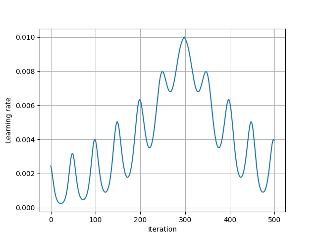
- class torchlib.optim.lr_scheduler.MountainLR(optimizer, total_epoch, peak_epoch, period_epoch, last_epoch=- 1)
Bases:
torch.optim.lr_scheduler._LRSchedulerSet the learning rate of each parameter group using a double gaussian kernel
\[(|x-P| / N) .* (-2 + cos(2 * (x-P) / T)) \]schedule, where \(\eta_{max}\) is set to the initial lr and \(T_{cur}\) is the number of epochs since the last restart in SGDR:
When last_epoch=-1, sets initial lr as lr. Notice that because the schedule is defined recursively, the learning rate can be simultaneously modified outside this scheduler by other operators.
The maximum learning rate are the base learning rate setted in Optimizer.
- Parameters
optimizer (Optimizer) – Wrapped optimizer.
t_eta_max (int) – Iterations when the learning rate reach to the maximum value \(\eta_{\max}\).
sigma1 (int) – Controls the shape of warming up phase.
sigma2 (int) – Controls the shape of annealing phase.
eta_start (float) – Starting learning rate. Default: 0.
eta_stop (float) – Stopping learning rate. Default: 0.
last_epoch (int) – The index of last epoch. Default: -1.
Examples

The results shown in the above figure can be obtained by the following codes.
import torch as th
import torchlib as tl
import matplotlib; matplotlib.use('TkAgg')
import matplotlib.pyplot as plt

lr = 1e-1
lr = 1e-2
# lr = 1e2

num_epochs = 1000
num_epochs = 500
batch_size = 8
num_batch = 750

params = {th.nn.parameter.Parameter(th.zeros(128), requires_grad=True),
        th.nn.parameter.Parameter(th.zeros(128), requires_grad=True),
        }

optimizer = th.optim.Adam(params, lr=lr)
scheduler = tl.optim.lr_scheduler.MountainLR(optimizer, total_epoch=num_epochs, peak_epoch=300, period_epoch=50, last_epoch=-1)

print(optimizer)

lrs = []
for n in range(num_epochs):
    for b in range(num_batch):

        optimizer.step()

        # lrs.append(optimizer.param_groups[0]['lr'])

    scheduler.step()
    lrs.append(optimizer.param_groups[0]['lr'])

plt.figure()
plt.plot(lrs)
plt.xlabel('Iteration')
plt.ylabel('Learning rate')
plt.grid()
plt.show()
- get_lr()
torchlib.optim.save_load module
- torchlib.optim.save_load.device_transfer(obj, name, device)